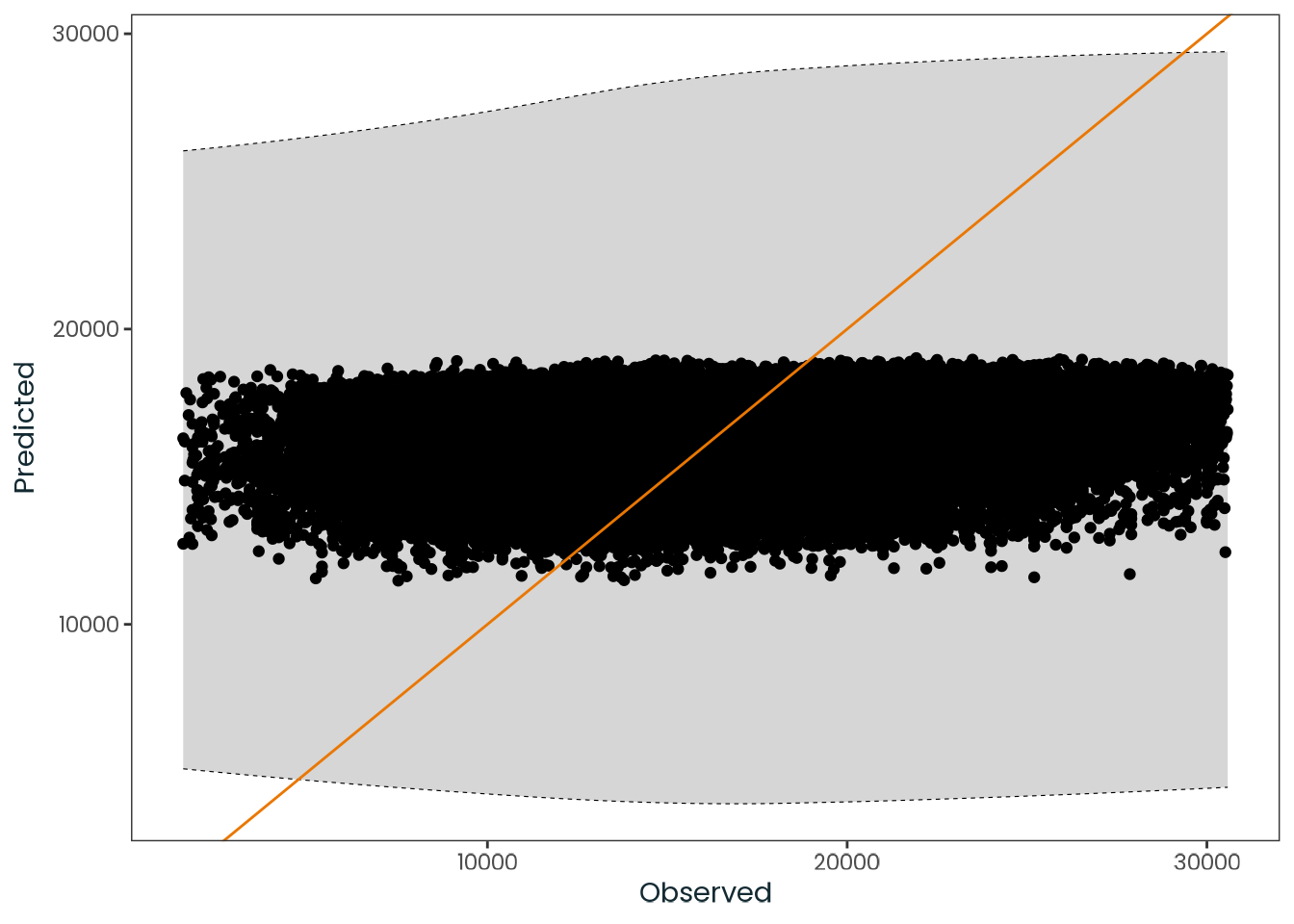
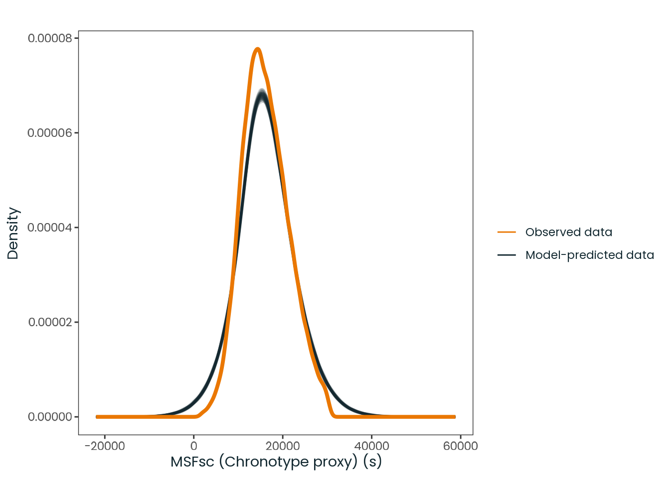
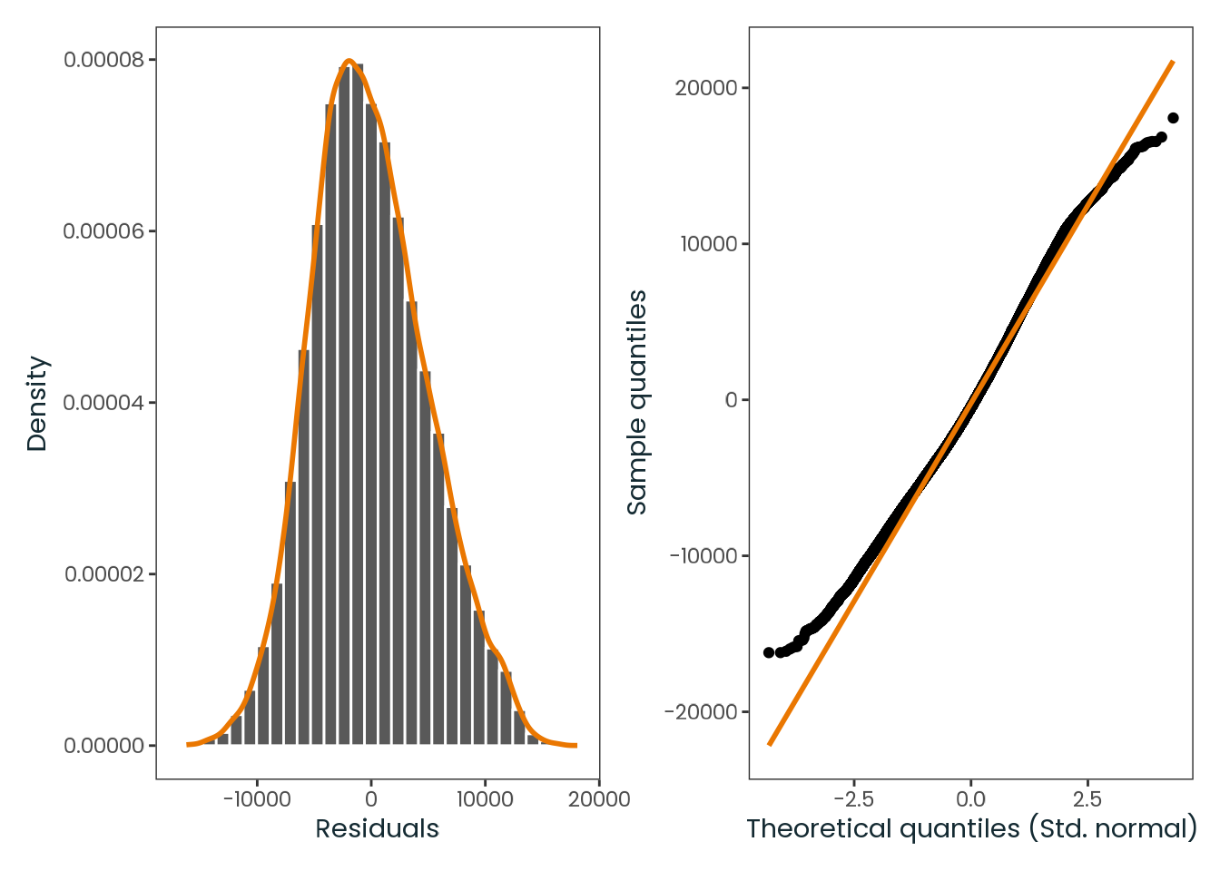
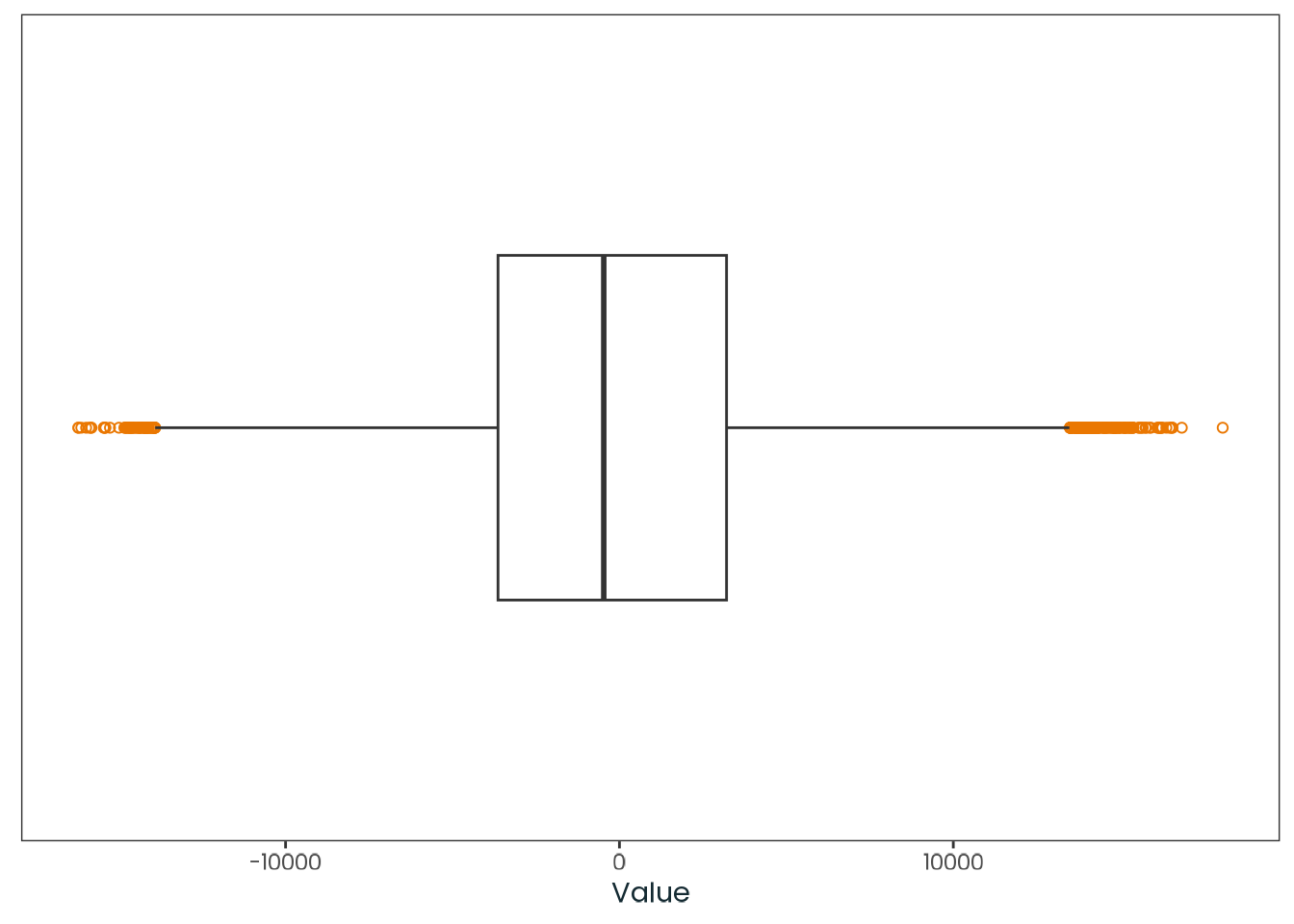
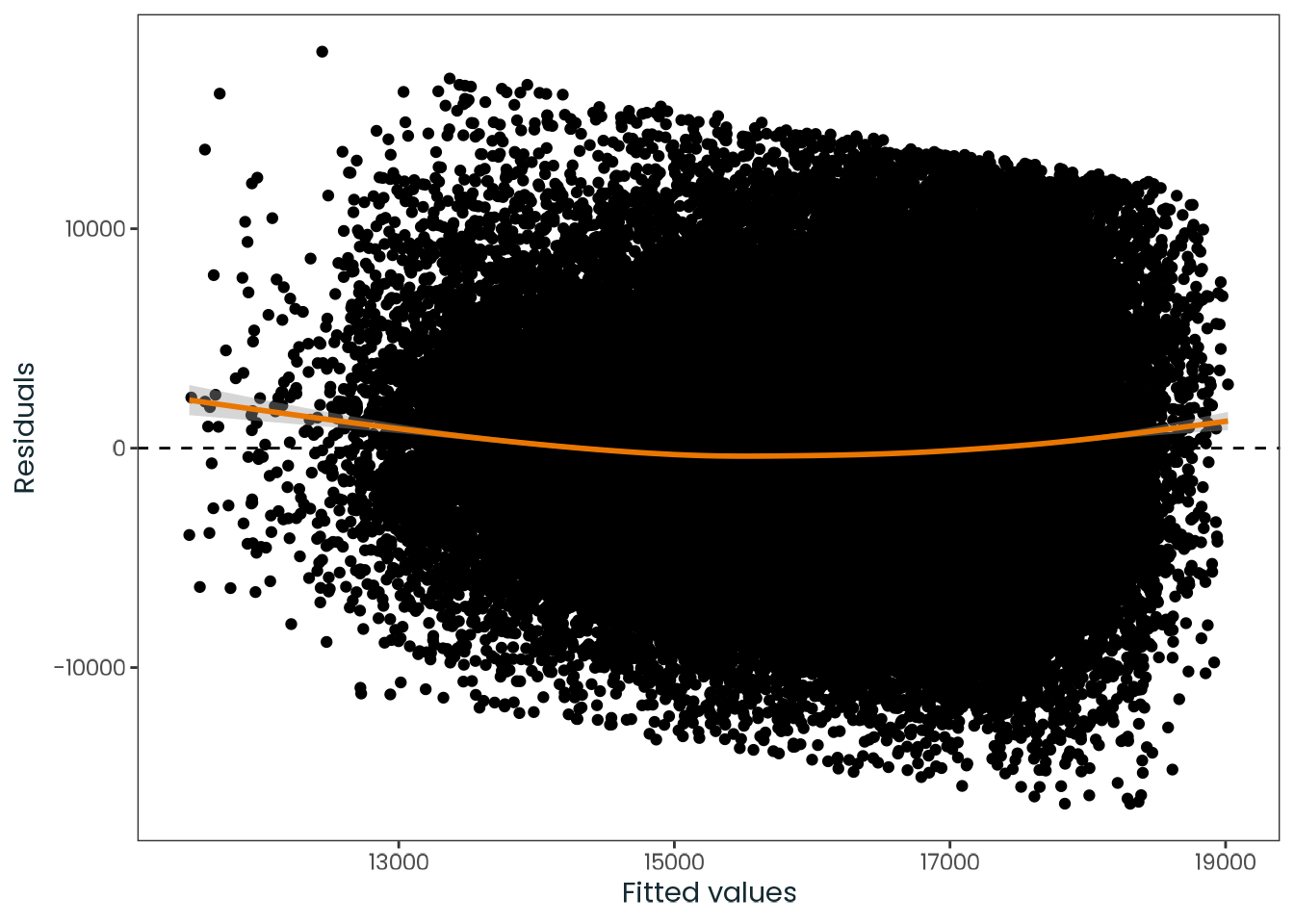
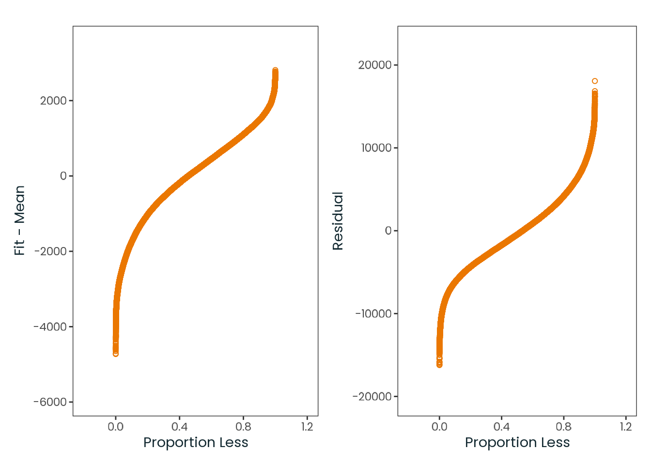
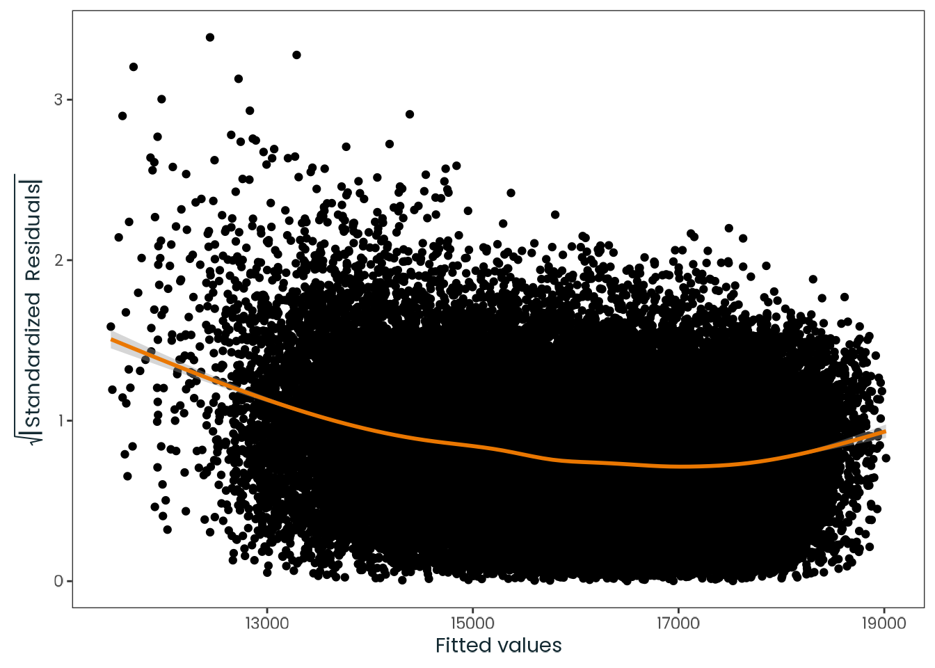
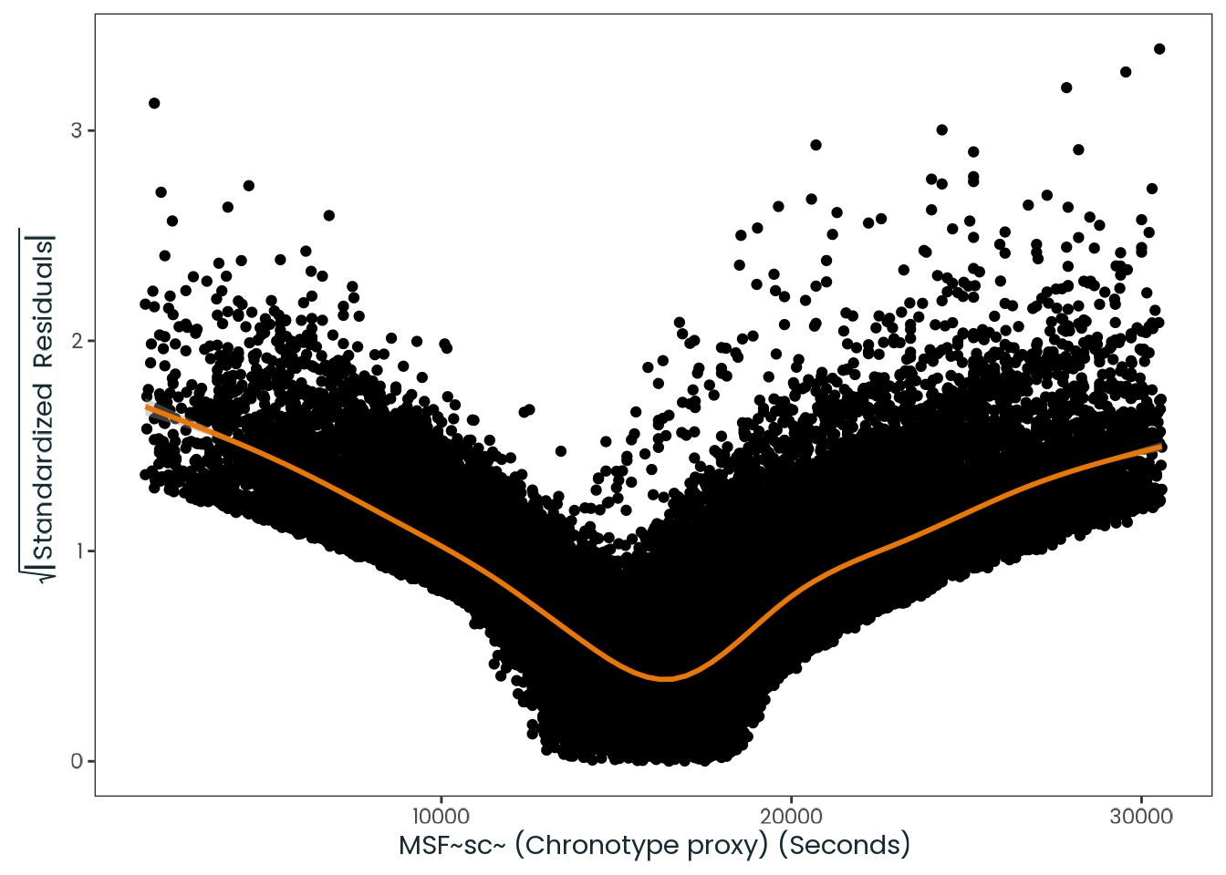
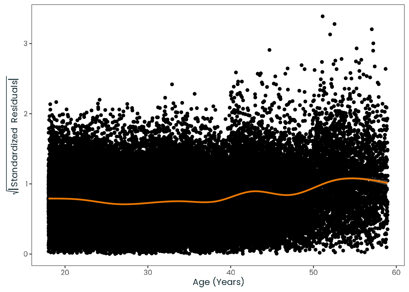
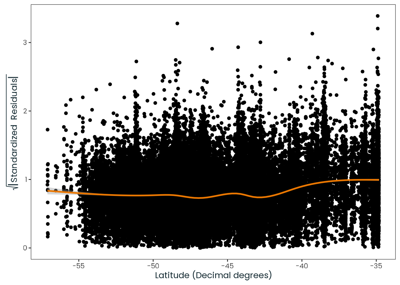
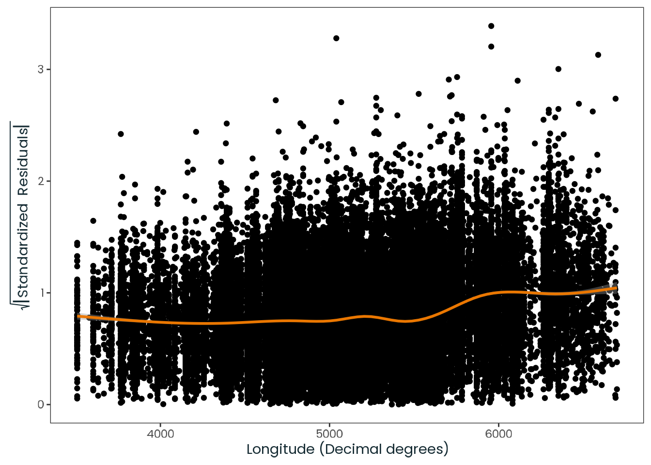
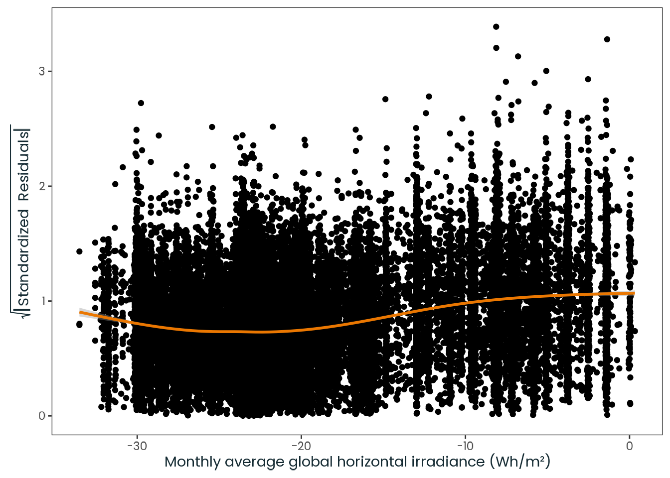
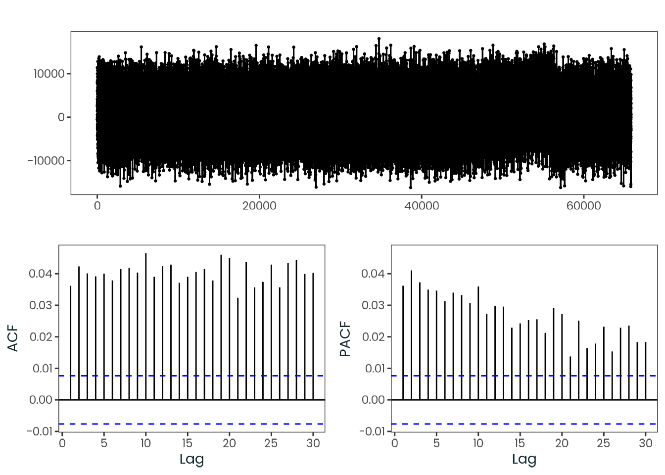
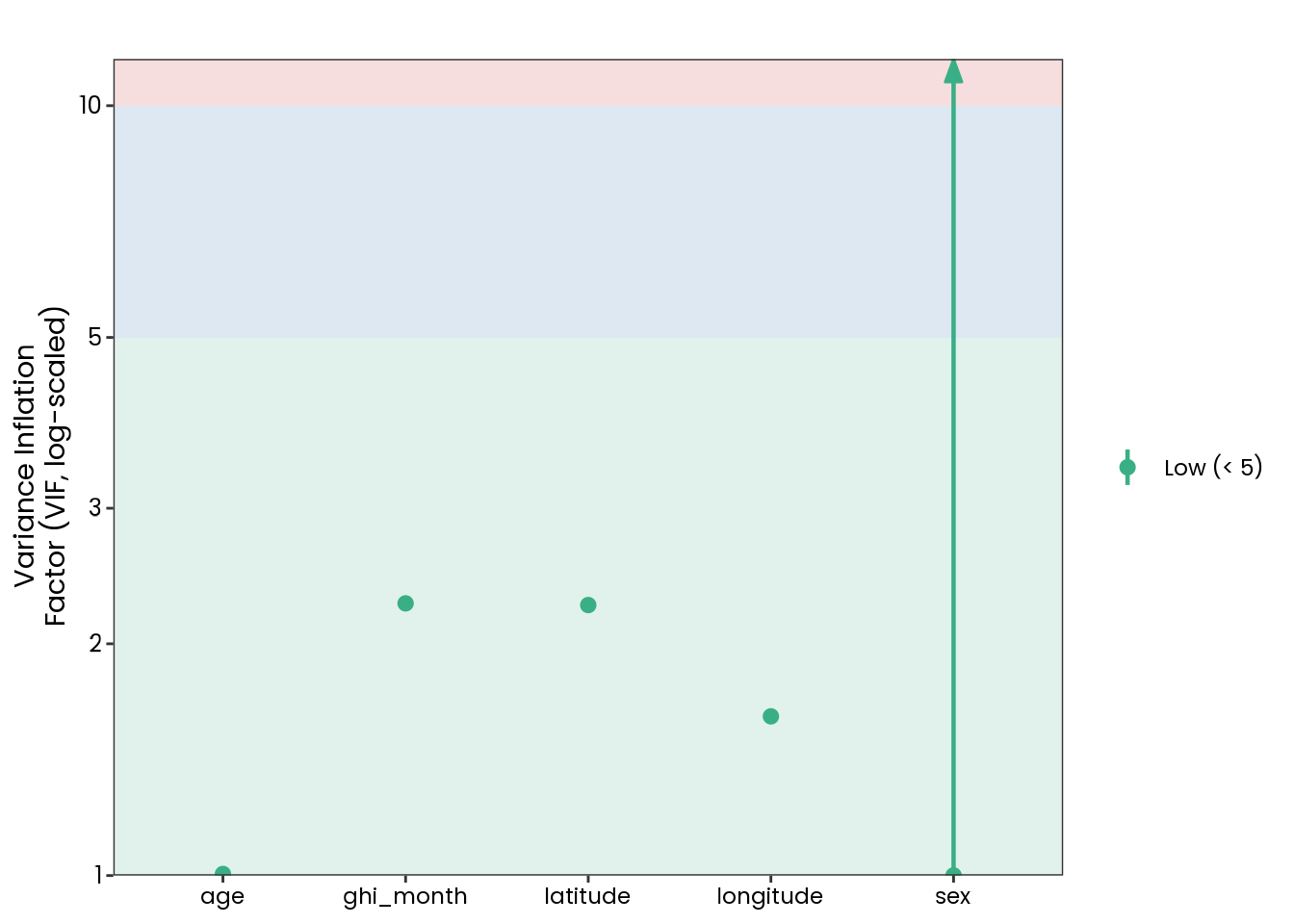
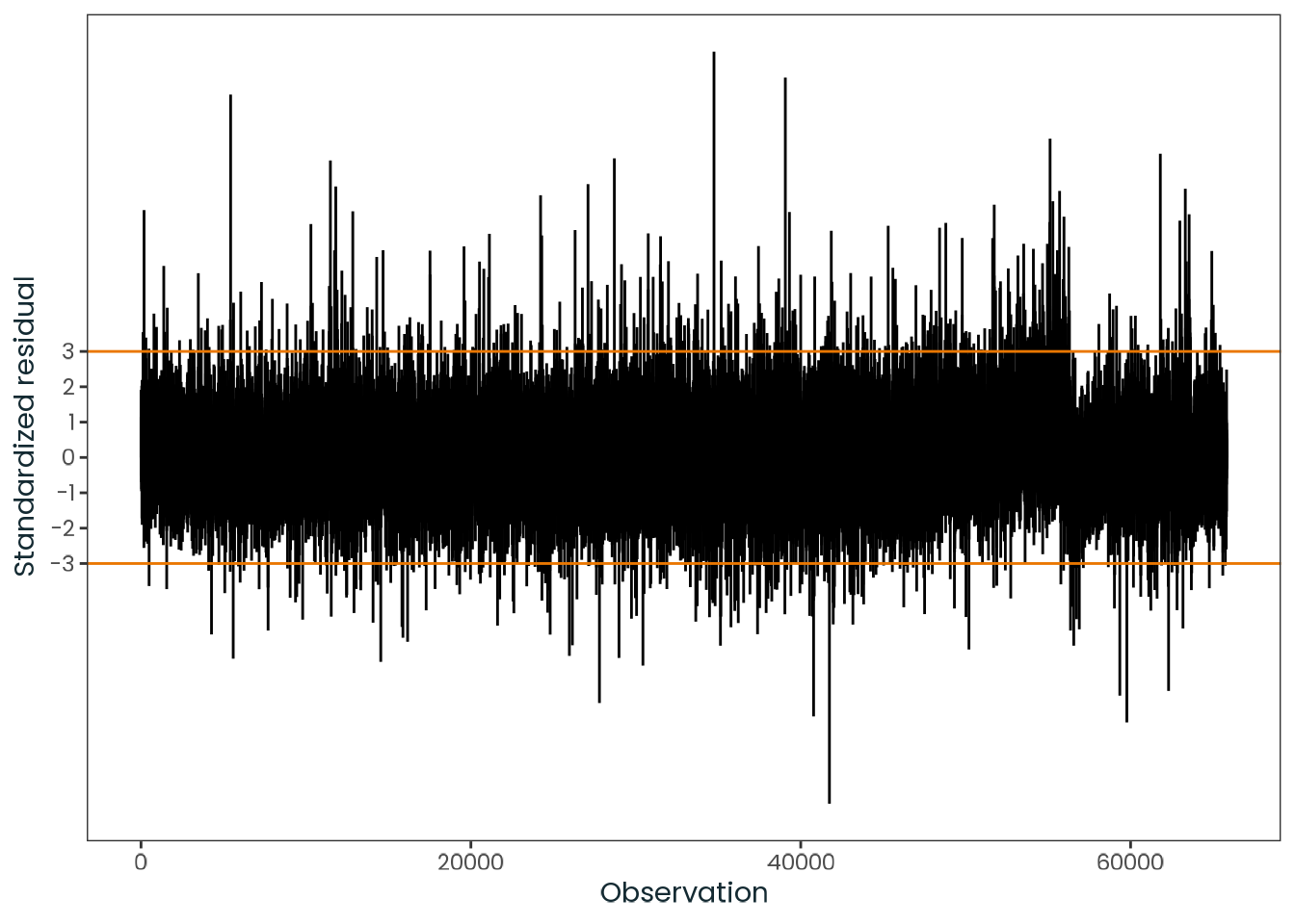
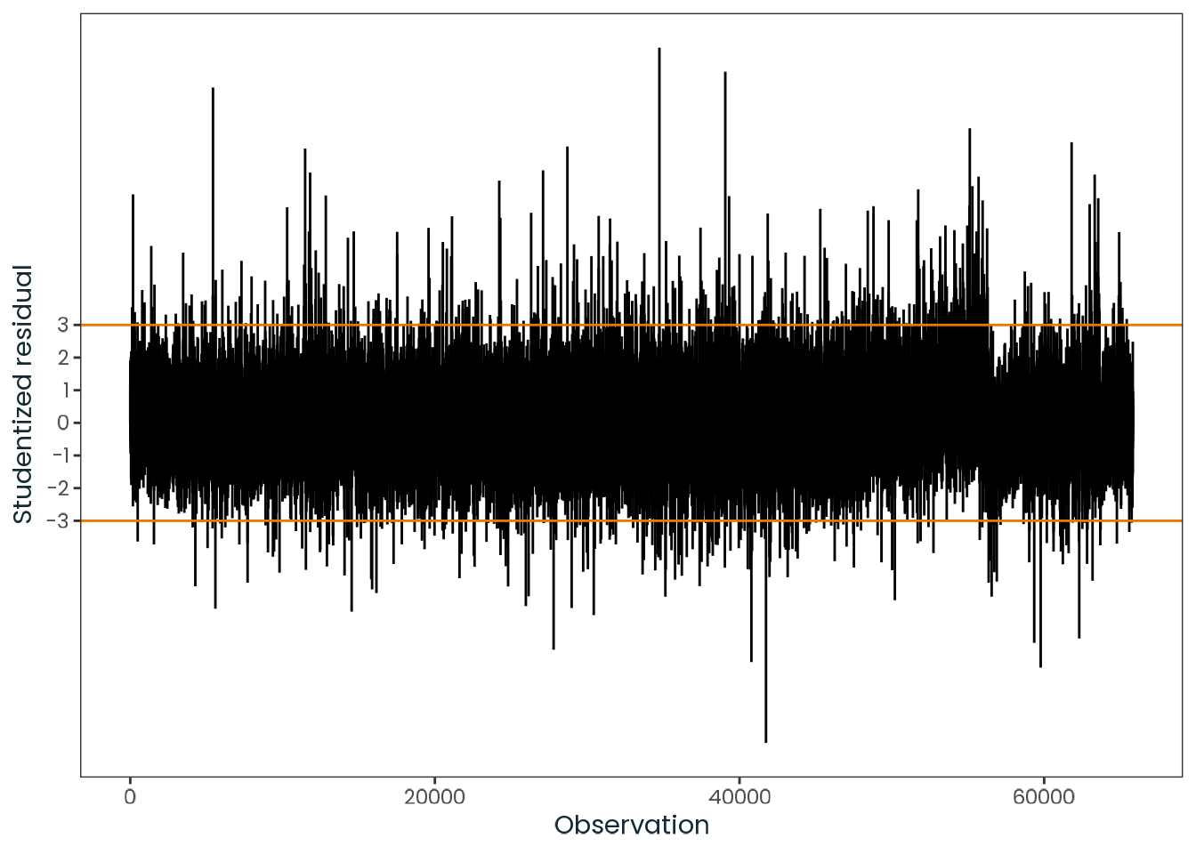
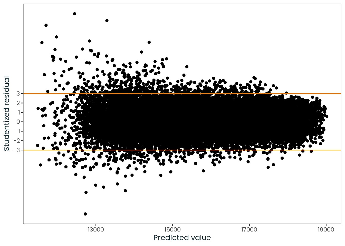
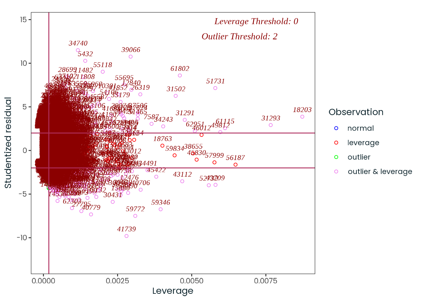
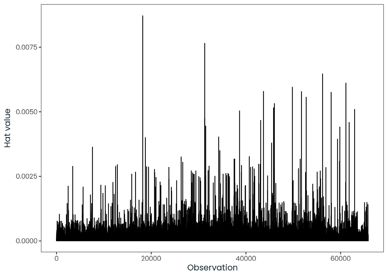
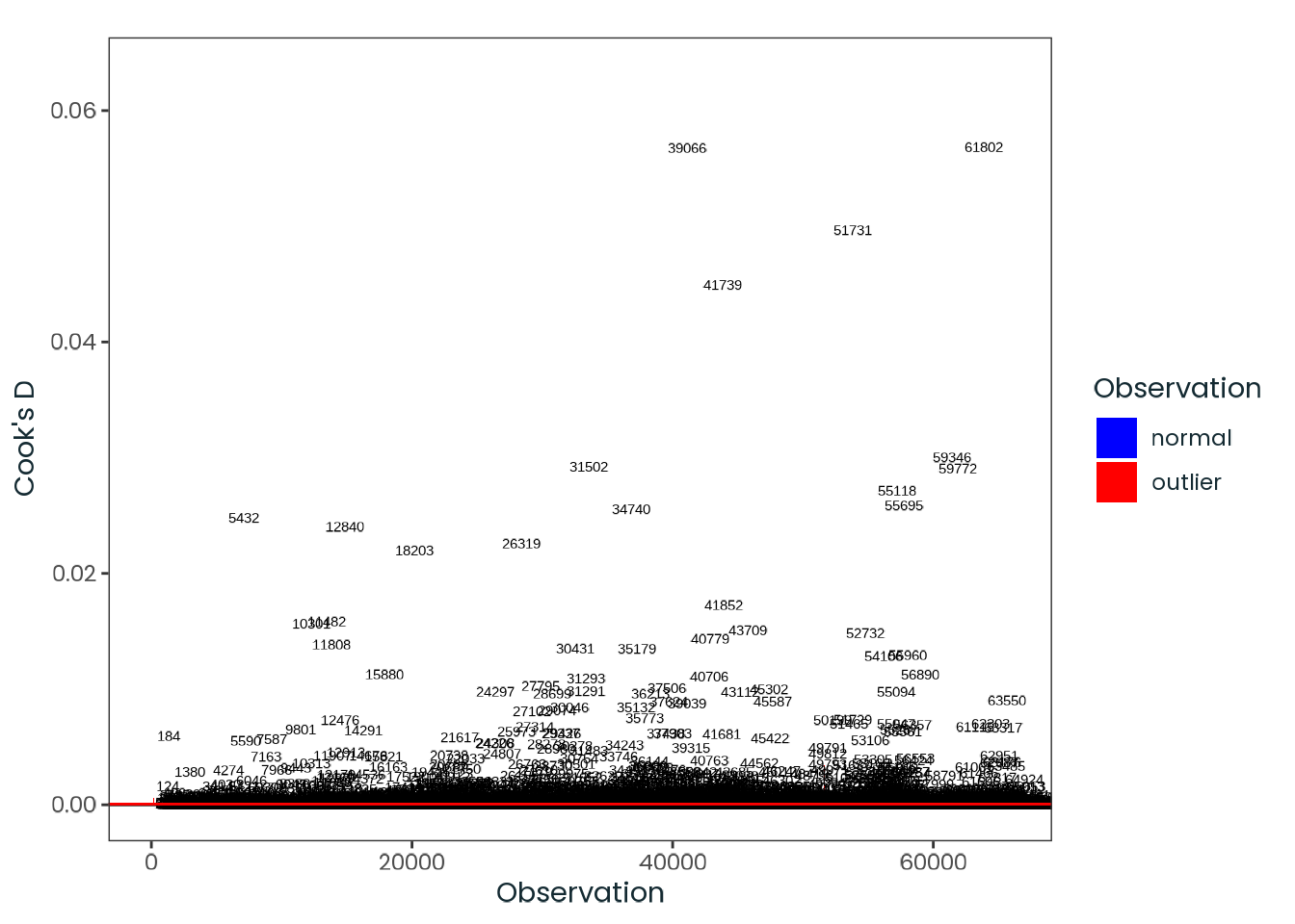
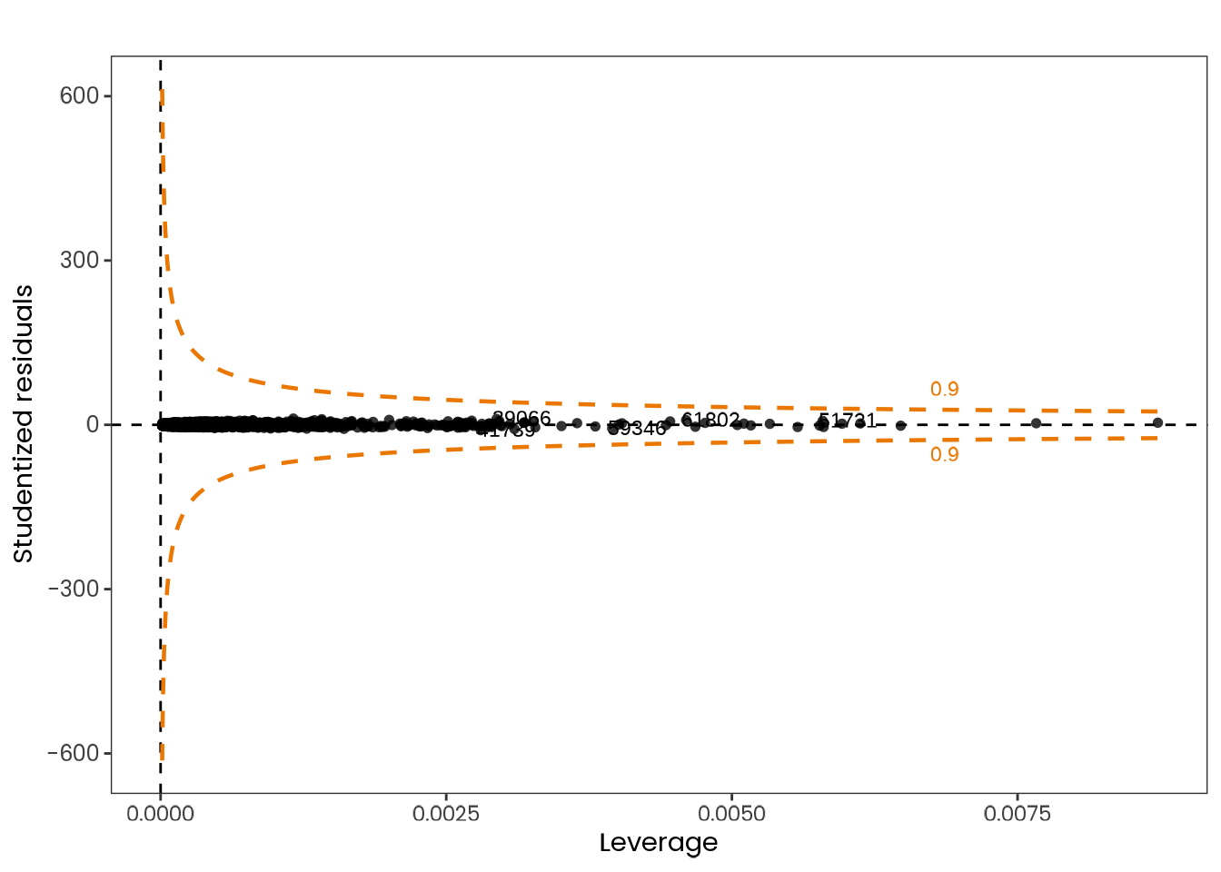
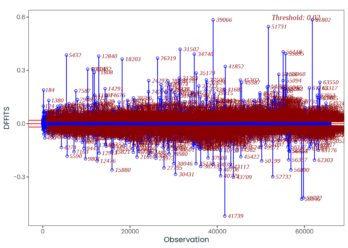
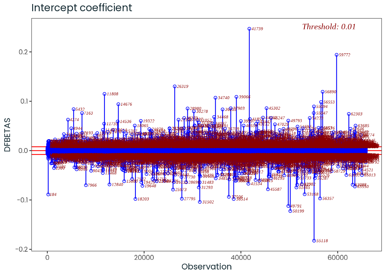
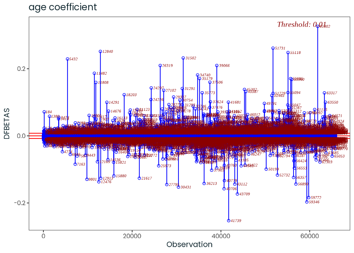
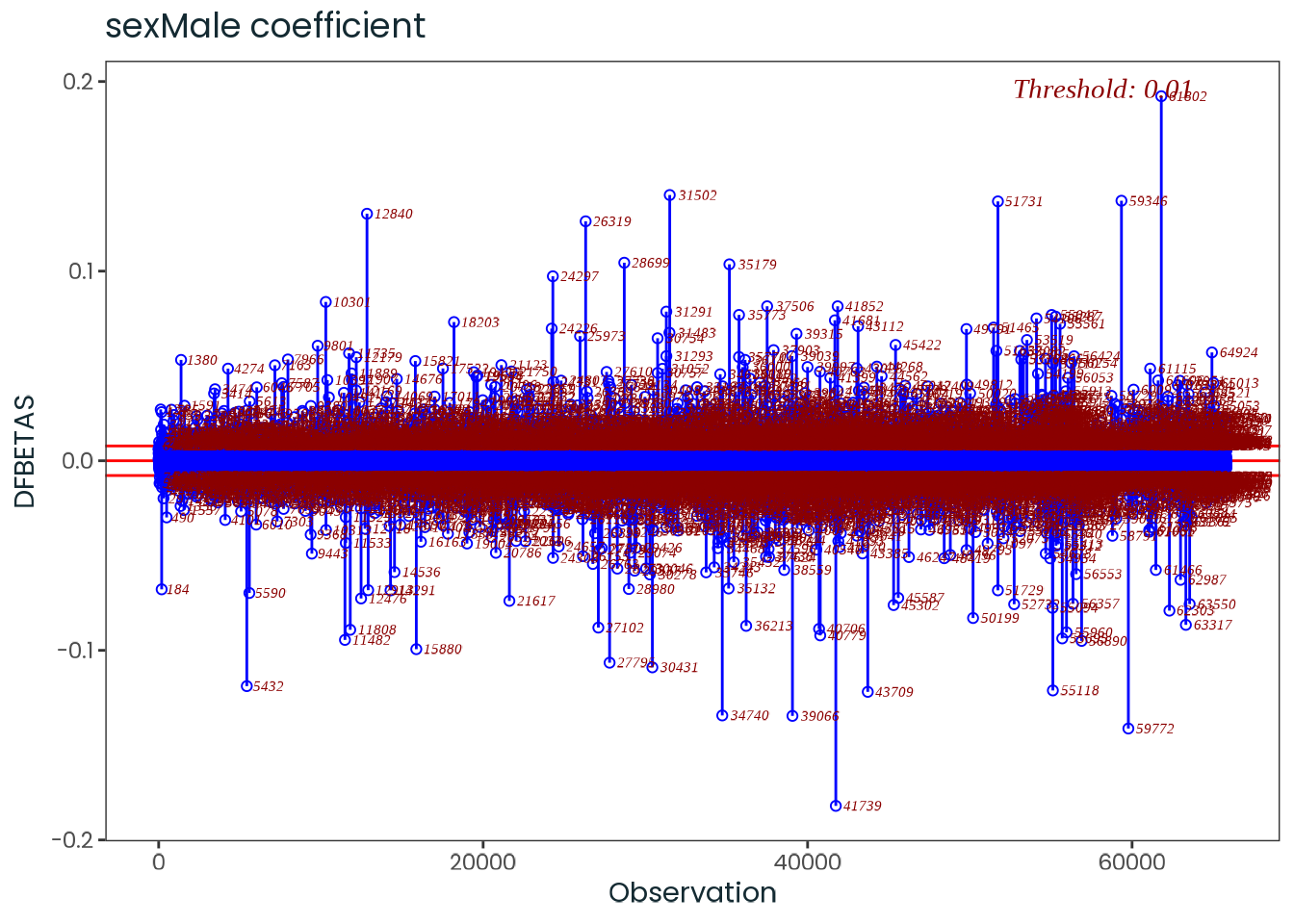
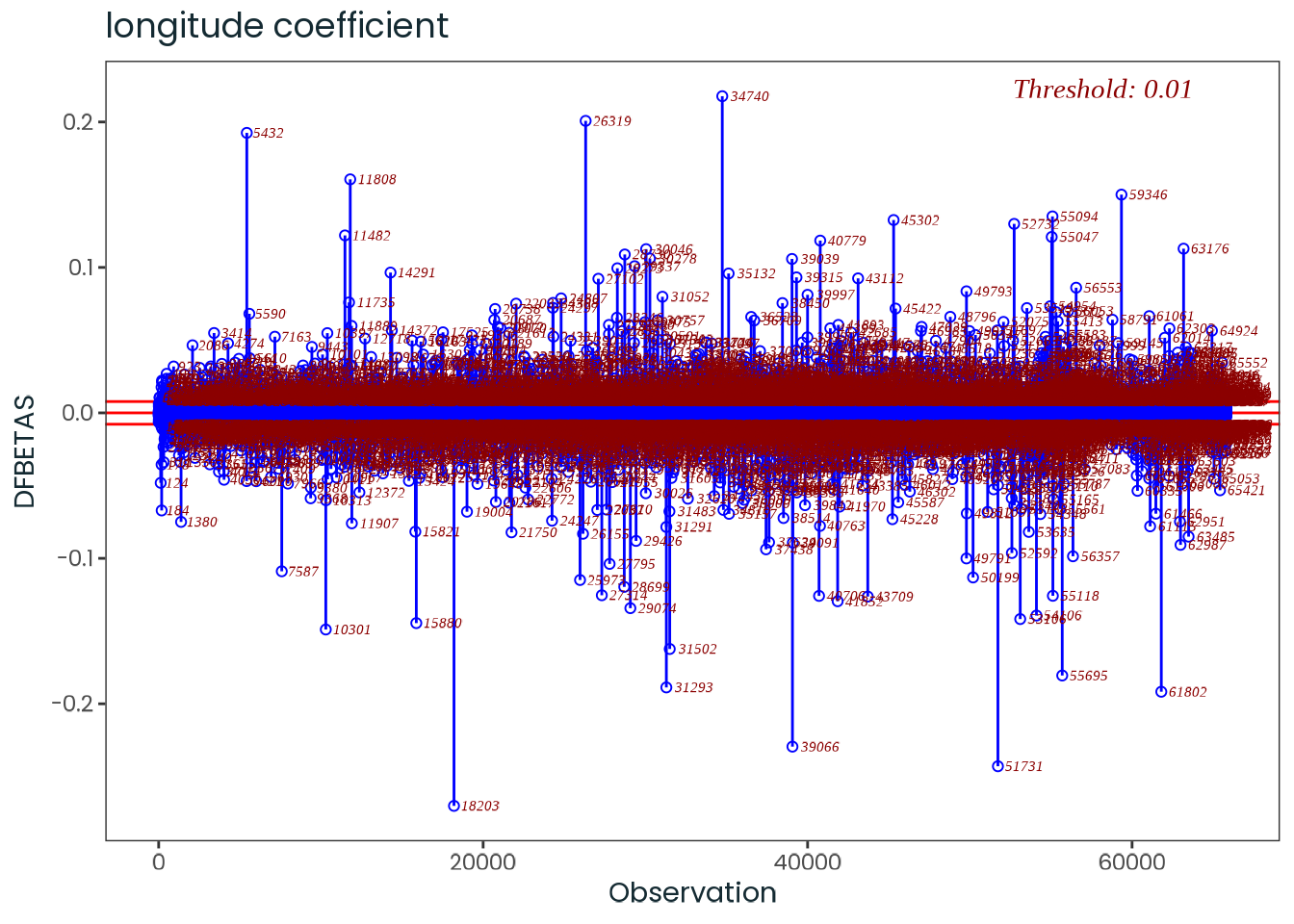
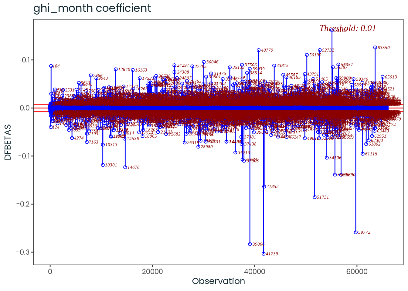
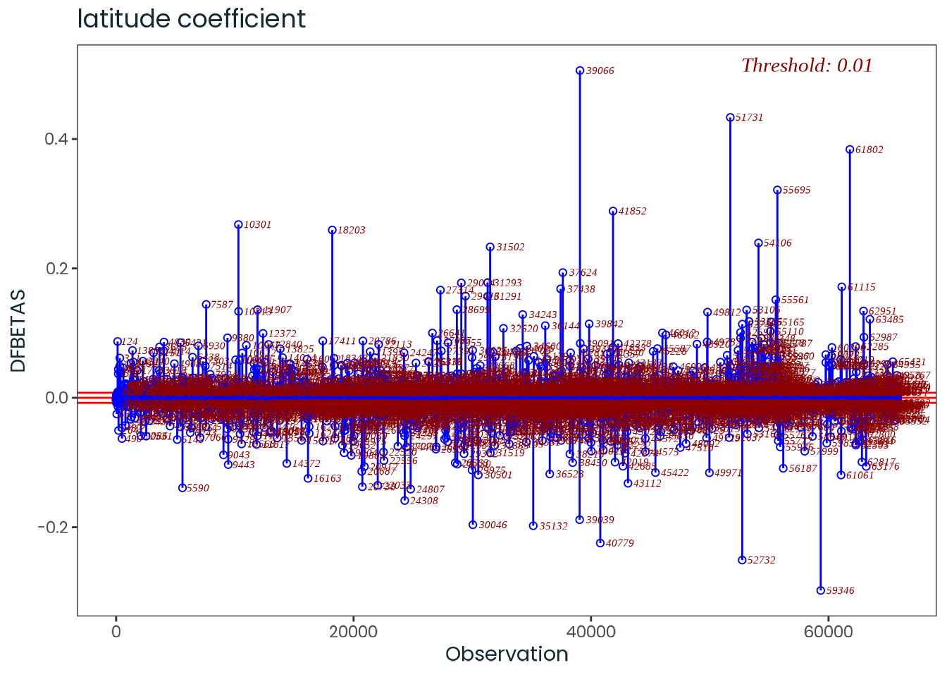
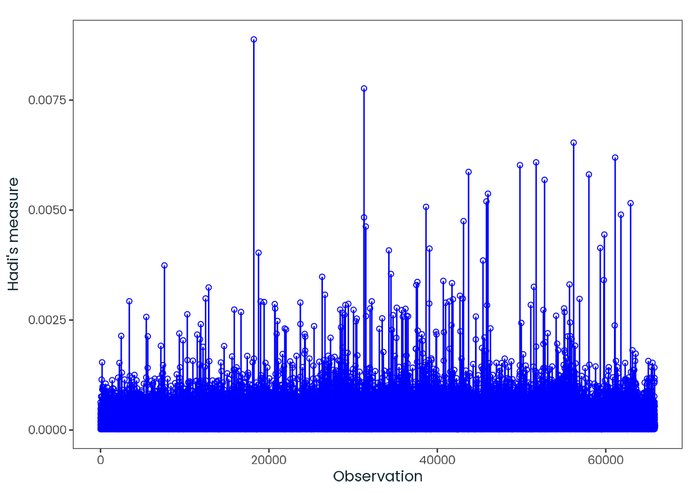
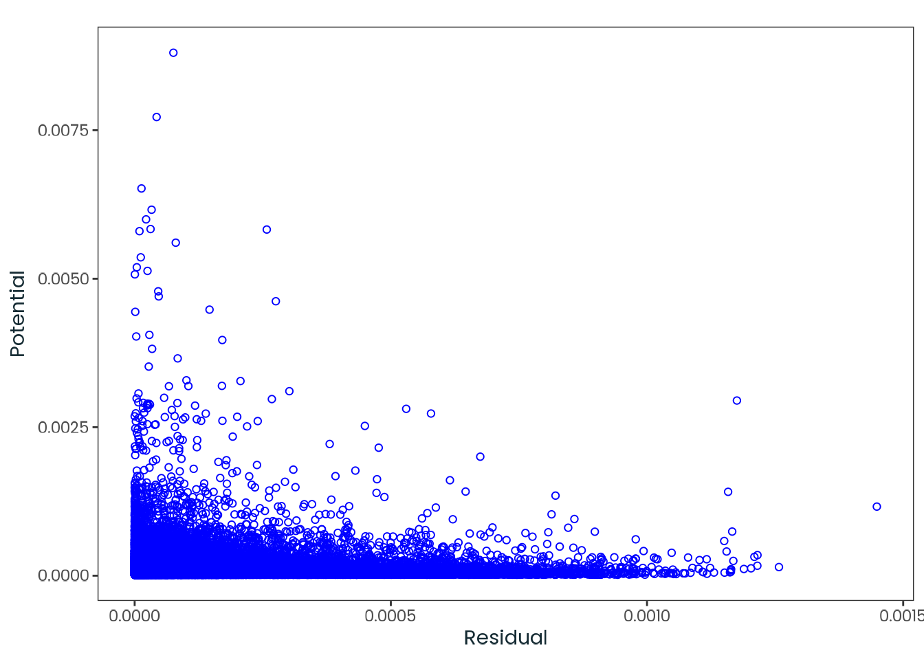
Based on the hypothesis test results and the methodology outlined in Supplementary Material B, we fail to reject the null hypothesis. Latitude does not meaningfully contribute to explaining the variance in chronotype.
Anderson, T. W. (1962). On the distribution of the two-sample
Cramér-von Mises criterion.
The Annals of Mathematical Statistics,
33(3), 1148–1159.
https://doi.org/10.1214/aoms/1177704477
Anderson, T. W., & Darling, D. A. (1952). Asymptotic theory of certain "goodness of fit" criteria based on stochastic processes.
The Annals of Mathematical Statistics,
23(2), 193–212.
https://www.jstor.org/stable/2236446
Anderson, T. W., & Darling, D. A. (1954). A test of goodness of fit.
Journal of the American Statistical Association,
49(268), 765–769.
https://doi.org/10.1080/01621459.1954.10501232
Belsley, D. A., Kuh, E., & Welsch, R. E. (2004).
Regression diagnostics: Identifying influential data and sources of collinearity (Print ISBN: 9780471058564
Online ISBN: 9780471725152). John Wiley & Sons.
https://doi.org/10.1002/0471725153
Bera, A. K., & Jarque, C. M. (1981). Efficient tests for normality, homoscedasticity and serial independence of regression residuals:
Monte Carlo evidence.
Economics Letters,
7(4), 313–318.
https://doi.org/10.1016/0165-1765(81)90035-5
Bonett, D. G., & Seier, E. (2002). A test of normality with high uniform power.
Computational Statistics & Data Analysis,
40(3), 435–445.
https://doi.org/10.1016/S0167-9473(02)00074-9
Box, G. E. P., & Pierce, D. A. (1970). Distribution of residual autocorrelations in autoregressive-integrated moving average time series models.
Journal of the American Statistical Association,
65(332), 1509–1526.
https://doi.org/10.1080/01621459.1970.10481180
Breusch, T. S., & Pagan, A. R. (1979). A simple test for heteroscedasticity and random coefficient variation.
Econometrica,
47(5), 1287–1294.
https://doi.org/10.2307/1911963
Chatterjee, S., & Hadi, A. S. (2012). Regression analysis by example (5th ed.). Wiley.
Cook, R. D. (1977). Detection of influential observation in linear regression.
Technometrics,
19(1), 15–18.
https://doi.org/10.1080/00401706.1977.10489493
Cook, R. D. (1979). Influential observations in linear regression.
Journal of the American Statistical Association,
74(365), 169–174.
https://doi.org/10.1080/01621459.1979.10481634
Cramér, H. (1928). On the composition of elementary errors:
First paper:
Mathematical deductions.
Scandinavian Actuarial Journal,
1928(1), 13–74.
https://doi.org/10.1080/03461238.1928.10416862
D’Agostino, R. B. (1971). An omnibus test of normality for moderate and large size samples.
Biometrika,
58(2), 341–348.
https://doi.org/10.1093/biomet/58.2.341
D’Agostino, R. B., & Belanger, A. (1990). A suggestion for using powerful and informative tests of normality.
The American Statistician,
44(4), 316–321.
https://doi.org/10.2307/2684359
D’Agostino, R. B., & Pearson, E. S. (1973). Tests for departure from normality.
Empirical results for the distributions of b2 and √b1.
Biometrika,
60(3), 613–622.
https://doi.org/10.1093/biomet/60.3.613
Dallal, G. E., & Wilkinson, L. (1986). An analytic approximation to the distribution of
Lilliefors’s test statistic for normality.
The American Statistician,
40(4), 294–296.
https://doi.org/10.1080/00031305.1986.10475419
DeGroot, M. H., & Schervish, M. J. (2012). Probability and statistics (OCLC: ocn502674206) (4th ed.). Addison-Wesley.
Durbin, J., & Watson, G. S. (1950). Testing for serial correlation in least squares regression.
I.
Biometrika,
37(3–4), 409–428.
https://doi.org/10.1093/biomet/37.3-4.409
Durbin, J., & Watson, G. S. (1951). Testing for serial correlation in least squares regression.
II.
Biometrika,
38(1–2), 159–178.
https://doi.org/10.1093/biomet/38.1-2.159
Durbin, J., & Watson, G. S. (1971). Testing for serial correlation in least squares regression.
III.
Biometrika,
58(1), 1–19.
https://doi.org/10.1093/biomet/58.1.1
Fox, J. (2016). Applied regression analysis and generalized linear models (3rd ed.). Sage.
Hair, J. F. (2019). Multivariate data analysis (8th ed.). Cengage.
Jarque, C. M., & Bera, A. K. (1980). Efficient tests for normality, homoscedasticity and serial independence of regression residuals.
Economics Letters,
6(3), 255–259.
https://doi.org/10.1016/0165-1765(80)90024-5
Jarque, C. M., & Bera, A. K. (1987). A test for normality of observations and regression residuals.
International Statistical Review,
55(2), 163–172.
https://doi.org/10.2307/1403192
Koenker, R. (1981). A note on studentizing a test for heteroscedasticity.
Journal of Econometrics,
17(1), 107–112.
https://doi.org/10.1016/0304-4076(81)90062-2
Kolmogorov, A. (1933). Sulla determinazione empirica di una legge di distribuzione. Giornale dell’Istituto Italiano degli Attuari, 4.
Kozak, M., & Piepho, H.-P. (2018). What’s normal anyway?
Residual plots are more telling than significance tests when checking
ANOVA assumptions.
Journal of Agronomy and Crop Science,
204(1), 86–98.
https://doi.org/10.1111/jac.12220
Lilliefors, H. W. (1967). On the
Kolmogorov-Smirnov test for normality with mean and variance unknown.
Journal of the American Statistical Association,
62(318), 399–402.
https://doi.org/10.1080/01621459.1967.10482916
Ljung, G. M., & Box, G. E. P. (1978). On a measure of lack of fit in time series models.
Biometrika,
65(2), 297–303.
https://doi.org/10.1093/biomet/65.2.297
Massey, F. J. (1951). The
Kolmogorov-Smirnov test for goodness of fit.
Journal of the American Statistical Association,
46(253), 68–78.
https://doi.org/10.1080/01621459.1951.10500769
Nahhas, R. W. (2024).
Introduction to regression methods for public health using R.
https://www.bookdown.org/rwnahhas/RMPH/
Newey, W. K., & West, K. D. (1987). A simple, positive semi-definite, heteroskedasticity and autocorrelation consistent covariance matrix.
Econometrica,
55(3), 703–708.
https://doi.org/10.2307/1913610
Newey, W. K., & West, K. D. (1994). Automatic lag selection in covariance matrix estimation.
The Review of Economic Studies,
61(4), 631–653.
https://doi.org/10.2307/2297912
Pearson, K. (1900). X.
On the criterion that a given system of deviations from the probable in the case of a correlated system of variables is such that it can be reasonably supposed to have arisen from random sampling.
The London, Edinburgh, and Dublin Philosophical Magazine and Journal of Science,
50(302), 157–175.
https://doi.org/10.1080/14786440009463897
Ramsey, J. B. (1969). Tests for specification errors in classical linear least-squares regression analysis.
Journal of the Royal Statistical Society. Series B (Methodological),
31(2), 350–371.
https://doi.org/10.1111/j.2517-6161.1969.tb00796.x
Schucany, W. R., & Ng, H. K. T. (2006). Preliminary goodness-of-fit tests for normality do not validate the one-sample
Student t.
Communications in Statistics - Theory and Methods,
35(12), 2275–2286.
https://doi.org/10.1080/03610920600853308
Shapiro, S. S., & Francia, R. S. (1972). An approximate analysis of variance test for normality.
Journal of the American Statistical Association,
67(337), 215–216.
https://doi.org/10.1080/01621459.1972.10481232
Shapiro, S. S., & Wilk, M. B. (1965). An analysis of variance test for normality (complete samples)†.
Biometrika,
52(3–4), 591–611.
https://doi.org/10.1093/biomet/52.3-4.591
Shatz, I. (2024). Assumption-checking rather than (just) testing:
The importance of visualization and effect size in statistical diagnostics.
Behavior Research Methods,
56(2), 826–845.
https://doi.org/10.3758/s13428-023-02072-x
Smirnov, N. (1948). Table for estimating the goodness of fit of empirical distributions. Annals of Mathematical Statistics, 19, 279–281.
Struck, J. (2024).
Regression Diagnostics with R. University of Wisconsin-Madison.
https://sscc.wisc.edu/sscc/pubs/RegDiag-R/
Thode, H. C. (2002). Testing for normality. Marcel Dekker.
Welsch, R., & Kuh, E. (1977).
Linear regression diagnostics (Working Paper 0173; p. 44). National Bureau of Economic Research.
https://doi.org/10.3386/w0173
