adj_r_squared_restricted <- rutils:::summarize_r2(
  r2 = 0.05964,
  n = 12845 + 8 + 1,
  k = 8,
  ci_level = 0.95,
  rules = "cohen1988"
)

adj_r_squared_restrictedAppendix K — Critique of Leocadio-Miguel et al. (2017)
K.1 Overview
This document presents a critique of the Leocadio-Miguel et al. (2017) article, aiming to contribute to the discussion of the latitude hypothesis, clarify the data presented, and highlight potential misinterpretations arising from the original analysis.
K.2 Inconsistent Data
We conducted a first regression of HO scores only on the covariates (age, longitude, and solar irradiation when the subjects filled the online questionnaire) and cofactors (sex, daylight saving time (DST), and season) (\(\text{R}^{2} = 0.05964\), \(\text{F}(8,12845) = 101.8\), \(p < 2.2e-16\)) (Leocadio-Miguel et al., 2017).
The \(\text{F}\)-test indicates \(8\) predictors, yet only \(6\) are mentioned in the text. This discrepancy is not clarified, leaving uncertainty about the additional predictors included in the model.
[continuing from the last quote] … and a second regression including the annual average solar irradiation, sunrise time, sunset time and daylight duration in March equinox, June, and December solstices for each volunteer (\(\text{R}^{2} = 0.06667\), \(\text{F}(27,12853) = 33.8\), \(p < 2.2e-16\)) (Leocadio-Miguel et al., 2017).
In this case, the \(\text{F}\)-test indicates \(27\) predictors. However, adding the \(8\) predictors from the first regression to the \(10\) newly mentioned variables yields a total of \(18\) predictors, not \(27\). This inconsistency is not addressed in the text.
Testing for nested models, we obtained a significant reduction of residual sum of squares (\(\text{F}(2,12884) = 31.983\), \(p = 1.395e-14\)), […] (Leocadio-Miguel et al., 2017).
The degrees of freedom difference (\(df = 2\)) suggests that the two previously described models were not directly compared in this nested test. This raises further questions about the models used, as the discrepancy is not explained.
K.3 Statistic Ritual
We also obtained an effect size estimate of Cohen’s \(f^{2} = (0.06352 - 0.05964) / (1 - 0.06352) = 0.004143174\) (Leocadio-Miguel et al., 2017).
A first thing to notice is that the higher \(\text{R}^{2}\) value (\(0.06352\)) differs from the previously reported \(\text{R}^{2}\) (\(0.06667\)). This inconsistency is not justified.
The formula that appears in the text is based on Cohen’s \(f^{2}\), which is calculated by the following:
\[ \text{Cohen's } f^2 = \cfrac{\text{R}^{2}}{1 - \text{R}^{2}} \]
For nested models, this can be adapted as:
\[ \text{Cohen's } f^2 = \cfrac{\text{R}^{2}_{f} - \text{R}^{2}_{r}}{1 - \text{R}^{2}_{f}} = \cfrac{\Delta \text{R}^{2}}{1 - \text{R}^{2}_{f}} \]
Before diving into the \(f^2\) calculation, let’s first calculate the confidence interval of the \(\text{R}^{2}\) for the restricted and full model using an estimate of the standard error. Note that all the parameters used in the calculations are provided in the text.
adj_r_squared_full <- rutils:::summarize_r2(
  r2 = 0.06352,
  n = 12853 + 27 + 1,
  k = 27,
  ci_level = 0.95,
  rules = "cohen1988"
)

adj_r_squared_full
Code
Based on this data, it’s also possible to estimate the confidence interval for the \(\Delta \text{R}^{2}\).
Code
rutils:::cohens_f_squared_summary(
  base_r_squared = adj_r_squared_restricted,
  new_r_squared = adj_r_squared_full
) |>
  rutils:::list_as_tibble()
As we can see, the authors found a negligible effect size, and its confidence interval even includes 0. Latitude-related predictors explained only \(0.388\%\) of the variability (\((0.06352 - 0.05964) \times 100\)). Despite this, the authors interpreted the result as evidence of an association.
At this point, the reader might ask: “If the effect size is so small, why was the F-test significant?”
Testing for nested models, we obtained a significant reduction of residual sum of squares (\(\text{F}(2,12884) = 31.983\), \(p = 1.395e-14\)), […] (Leocadio-Miguel et al., 2017).
The significant \(p\)-value found in their F-test for nested models indicate a difference only because the \(p\)-value is very sensitive to sample size (\(12,884\), in their case) (Figure K.1). This is a common issue in large samples (commonly called the “\(p\)-value problem”), where even small differences (e.g., a difference of \(0.00001\)) can be detected as significant (Lin et al., 2013).
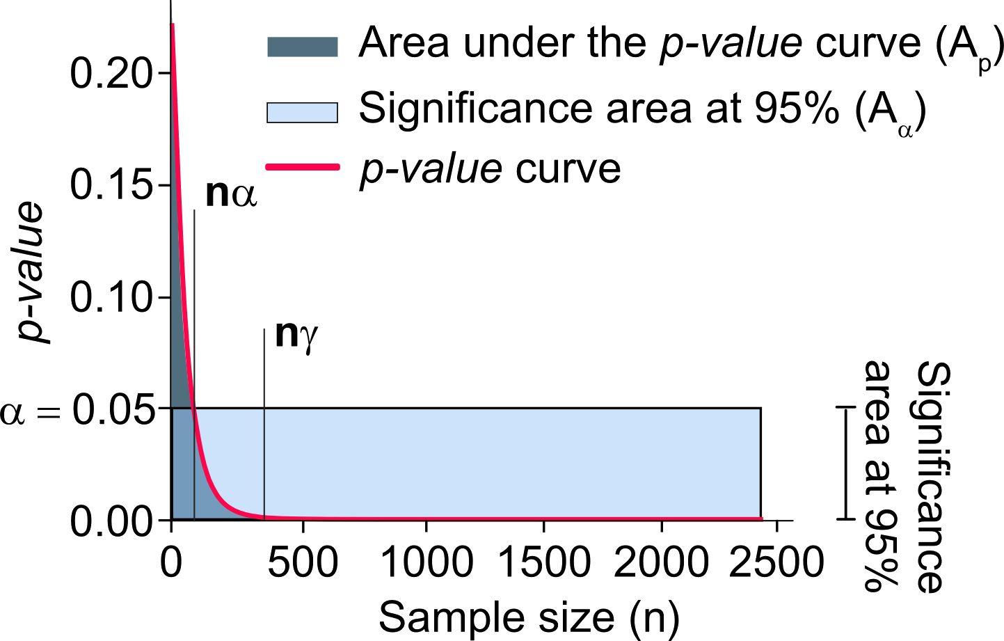
Source: Reproduced from Gómez-de-Mariscal et al. (2021, Figure 3).
A \(p\)-value do not have any practical significance, that is why the effect size is important. As Cohen (1988, p. 461) put:
[…] in many circumstances, all that is intended by “proving” the null hypothesis is that the ES [Effect Size] is not necessarily zero but small enough to be negligible.
Authors who rely solely on \(p\)-values demonstrate a statistical ritual rather than engaging in statistical thinking (Gigerenzer, 2004).
K.4 Model Issues
We tested the residuals of the second regression with Kolmogorov-Smirnov normality test and obtained a significant result (\(\text{D} = 0.42598\), \(p < 2.2e-16\)) (Leocadio-Miguel et al., 2017).
This result violates the assumptions of linear regression and it’s not addressed in the text.
Objective assumption tests (e.g., Anderson–Darling test) is not advisable for larger samples, since they can be overly sensitive to minor deviations. Additionally, they might overlook visual patterns that are not captured by a single metric (Kozak & Piepho, 2018; Schucany & Ng, 2006; Shatz, 2024).
Nevertheless, the authors did not mention this in the text.
The irradiation (W/m2) data by latitude was acquired from the NASA website (http://aom.giss.nasa.gov). We retrieved monthly average data and calculated the annual mean for each latitude degree (Leocadio-Miguel et al., 2017).
The type of irradiation (e.g., global, direct, or diffuse) was not specified, nor was it included in the supplementary materials. This omission is crucial, as different irradiation types can yield substantially different results.
[…] a second regression including the annual average solar irradiation, sunrise time, sunset time and daylight duration in March equinox, June, and December solstices for each volunteer (Leocadio-Miguel et al., 2017).
The inclusion of sunrise time, sunset time, and daylight duration (sunset - sunrise) likely introduced multicollinearity due to their inherent correlation. The study does not acknowledge or address this potential issue.
K.5 Misleading Visualization
The Figure 2 shown in Leocadio-Miguel et al. (2017) provides a good example of how data can be misleading. This Figure was shown many times in presentations in chronobiology symposiums, without a proper care of understanding what it was showing.
To interpret this figure, it is essential to first comprehend the scale it represents. In Leocadio-Miguel et al. (2017), the authors used the Horne & Östberg (HO) chronotype scale (Horne & Östberg, 1976) (Figure K.2). This scale, one of the first developed to assess chronotype, is a self-report questionnaire designed to determine an individual’s preferred time of day for activities such as waking up, going to bed, and moment of peak performance. The HO scale consists of \(19\) items, with a total score ranging from \(16\) to \(86\). Lower scores indicate greater evening orientation, while higher scores reflect stronger morning orientation(Table K.1).
Code
Source: Adapted from Horne & Östberg (1976).
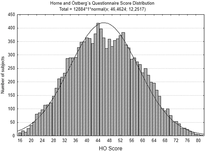
Source: Reproduced from Leocadio-Miguel et al. (2017, Figure 1).
K.5.1 The Figure
One of the key issues with the data presented in Leocadio-Miguel et al. (2017) is that it relies on negligible associations, yet the authors present them in a way that suggests a strong effect. The article’s Figure 2 (Figure K.3) illustrates this. At first glance, it appears to show a good fit and a strong relationship between latitude and the chronotype proxy (in this case, the HO score). However, a closer analysis reveals that it is a clear example of the \(y\)-axis illusion.
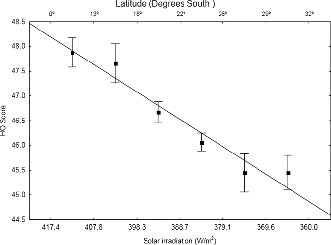
Source: Reproduced from Leocadio-Miguel et al. (2017, Figure 2).
In the following sections, the data extracted from the figure is reproduced to provide a more accurate and transparent representation of the relationship reported by the authors.
K.5.2 Latitude Estimation (Upper \(x\)-Axis)
As shown in Figure K.4, the latitude does not follow a fixed scale. Instead, it is referenced relative to the second \(x\)-axis (Solar irradiation). However, it is possible to estimate the latitude values reasonably well by measuring the pixel distances between points on the figure.
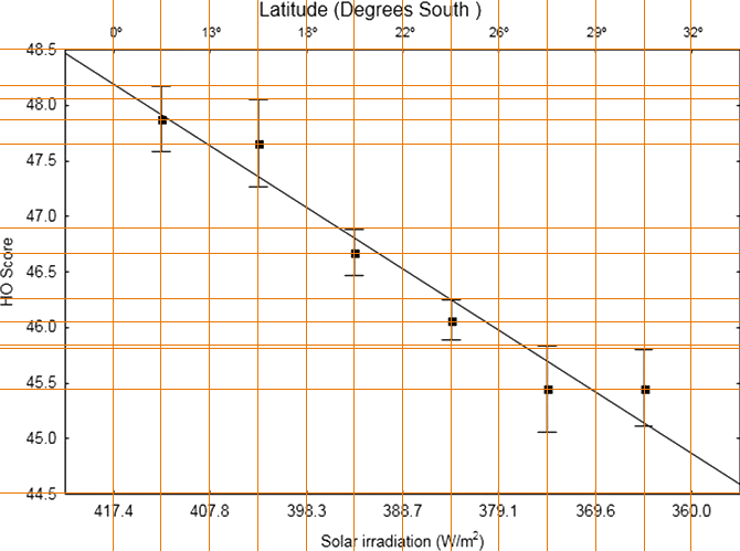
Source: Adapted by the author from Leocadio-Miguel et al. (2017, Figure 2).
Interval distances
- \(0\text{-}13\): \(87\) pixels. \(87 / 13\): 1 point \(\approx 6.692308\) pixels.
- \(13\text{-}18\): \(88\) pixels. \(88 / (18 - 13)\): \(1\) point \(= 17.6\) pixels.
- \(18\text{-}22\): \(87\) pixels. \(87 / (22 - 18)\): \(1\) point \(= 21.75\) pixels.
- \(22\text{-}26\): \(87\) pixels. \(87 / (26 - 22)\): \(1\) point \(= 21.75\) pixels.
- \(26\text{-}29\): \(88\) pixels. \(88 / (29 - 26)\): \(1\) point \(\approx 29.333\) pixels.
- \(29\text{-}32\): \(86\) pixels. \(86 / (32 - 29)\): \(1\) point \(\approx 28.667\) pixels.
Estimation
- 1st point: \(0\) to point: \(42\) pixels. Estimation: \(42 / (87 / 13) \approx 6.275862\).
- 2nd point: \(13\) to point: \(44\) pixels. Estimation: \(13 + (44 / (88 / (18 - 13))) = 15.5\).
- 3rd point: \(18\) to point: \(43\) pixels. Estimation: \(18 + (43 / (87 / (22 - 18))) \approx 19.97701\).
- 4th point: \(22\) to point: \(44\) pixels. Estimation: \(22 + (44 / (87 / (26 - 22))) \approx 24.02299\).
- 5th point: \(26\) to point: \(44\) pixels. Estimation: \(26 + (44 / (87 / (29 - 26))) \approx 27.51724\).
- 6th point: \(29\) to point: \(44\) pixels. Estimation: \(29 + (44 / (86 / (32 - 29))) \approx 30.53488\).
K.5.3 HO Estimation (\(y\)-Axis)
The HO value scale is fixed, allowing the values to be accurately determined by measuring the pixel distances.
Pixel/Point
- \(44.5\text{-}48.5\): \(402\) pixels. \(402 / (48.5 - 44.5)\): \(1\) point \(= 100.5\) pixels.
Estimation
- 1st point: \(44.5\) to point: \(338\) pixels. Estimation: \(44.5 + (338 / (402 / (48.5 - 44.5))) \approx 47.86318\).
- 2nd point: \(44.5\) to point: \(316\) pixels. Estimation: \(44.5 + (316 / (402 / (48.5 - 44.5))) \approx 47.64428\).
- 3rd point: \(44.5\) to point: \(217\) pixels. Estimation: \(44.5 + (217 / (402 / (48.5 - 44.5))) \approx 46.6592\).
- 4th point: \(44.5\) to point: \(155\) pixels. Estimation: \(44.5 + (155 / (402 / (48.5 - 44.5))) \approx 46.04229\).
- 5th point: \(44.5\) to point: \(94\) pixels. Estimation: \(44.5 + (94 / (402 / (48.5 - 44.5))) \approx 45.43532\).
- 6th point: \(44.5\) to point: \(94\) pixels. Estimation: \(44.5 + (94 / (402 / (48.5 - 44.5))) \approx 45.43532\).
K.5.4 Standard Error Estimation (\(y\)-Axis)
The standard error (SE) is displayed on the \(y\)-axis, which has a fixed scale. Therefore, the values can be accurately determined by measuring the pixel distances.
Pixel/Point
- \(44.5\text{-}48.5\): \(402\) pixels. \(402 / (48.5 - 44.5)\): \(1\) point \(= 100.5\) pixels.
Estimation
- 1st point SE: \(44.5\) to upper SE: \(369\) pixels. Estimation: \(44.5 + (369 / (402 / (48.5 - 44.5))) \approx 48.17164\).
- 2nd point SE: \(44.5\) to upper SE: \(357\) pixels. Estimation: \(44.5 + (357 / (402 / (48.5 - 44.5))) \approx 48.05224\).
- 3rd point SE: \(44.5\) to upper SE: \(240\) pixels. Estimation: \(44.5 + (240 / (402 / (48.5 - 44.5))) \approx 46.88806\)
- 4th point SE: \(44.5\) to upper SE: \(176\) pixels. Estimation: \(44.5 + (176 / (402 / (48.5 - 44.5))) \approx 46.25124\)
- 5th point SE: \(44.5\) to upper SE: \(134\) pixels. Estimation: \(44.5 + (134 / (402 / (48.5 - 44.5))) \approx 45.83333\)
- 6th point SE: \(44.5\) to upper SE: \(131\) pixels. Estimation: \(44.5 + (131 / (402 / (48.5 - 44.5))) \approx 45.80348\)
K.5.5 The Extracted Data
By following the process described above, we can obtain a reliable approximation of the data, as shown below.
Code
data <-
  dplyr::tibble(
    ho = c(
      44.5 + (338 / (402 / (48.5 - 44.5))),
      44.5 + (316 / (402 / (48.5 - 44.5))),
      44.5 + (217 / (402 / (48.5 - 44.5))),
      44.5 + (155 / (402 / (48.5 - 44.5))),
      44.5 + (94 / (402 / (48.5 - 44.5))),
      44.5 + (94 / (402 / (48.5 - 44.5)))
    ),
    latitude = c(
      42 / (87 / 13),
      13 + (44 / (88 / (18 - 13))),
      18 + (43 / (87 / (22 - 18))),
      22 + (44 / (87 / (26 - 22))),
      26 + (44 / (87 / (29 - 26))),
      29 + (44 / (86 / (32 - 29)))
    )
  ) |>
  dplyr::mutate(
    se_upper = c(
      44.5 + (369 / (402 / (48.5 - 44.5))),
      44.5 + (357 / (402 / (48.5 - 44.5))),
      44.5 + (240 / (402 / (48.5 - 44.5))),
      44.5 + (176 / (402 / (48.5 - 44.5))),
      44.5 + (134 / (402 / (48.5 - 44.5))),
      44.5 + (131 / (402 / (48.5 - 44.5)))
    ),
    se = se_upper - ho
  )

dataSource: Created by the author, based on a data extracted from Leocadio-Miguel et al. (2017, Figure 2).
K.5.6 Plotting the Extracted Data
First, let’s examine the data in a format similar to what is shown in the Leocadio-Miguel et al. (2017) figure.
Here, the \(x\)-axis follows a fixed scale, ensuring an accurate and distortion-free representation of the data.
Code
data |>
  ggplot2::ggplot(
    ggplot2::aes(x = latitude, y = ho)
  ) +
  ggplot2::geom_point(shape = 15, size = 3) +
  ggplot2::geom_errorbar(
    ggplot2::aes(
      x = latitude,
      y = ho,
      ymin = ho - se,
      ymax= ho + se
    ),
    data = data,
    show.legend = FALSE,
    inherit.aes = FALSE,
    width = 0.5,
    linewidth = 0.5
  ) +
  ggplot2::geom_smooth(
    method = "lm",
    formula = y ~ x,
    se = FALSE,
    color = brandr::get_brand_color("orange"),
    linewidth = 2
  ) +
  ggplot2::scale_x_continuous(
    breaks = c(0, 13, 18, 22, 26, 29, 32),
    labels = c("0º", "13º", "18º", "22º", "26º", "29º", "32º"),
    limits = c(0, 32)
  ) +
  ggplot2::labs(
    x = "Latitude (Degrees South)",
    y = "HO Score"
  )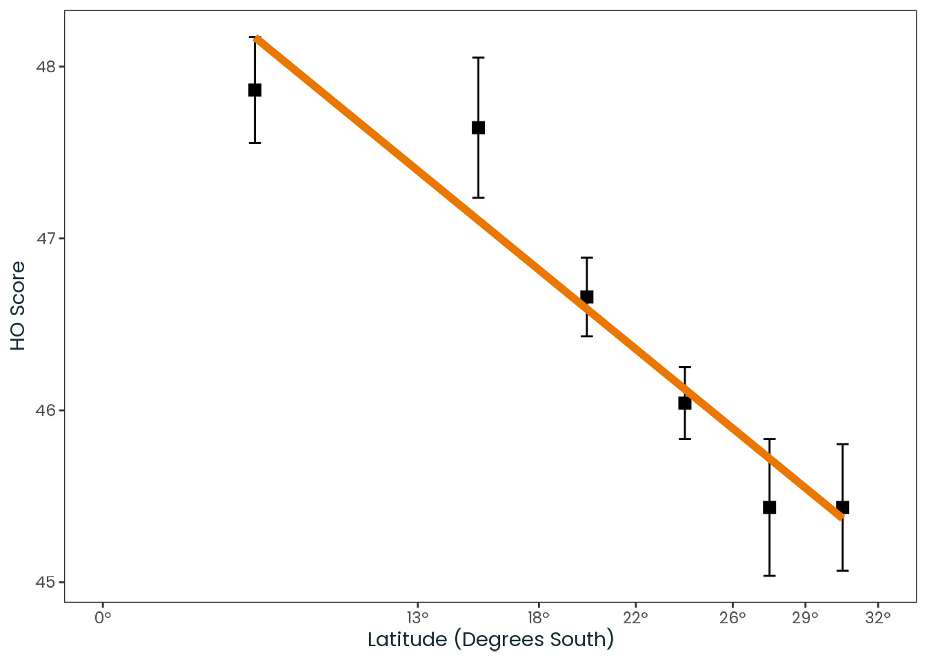
Source: Created by the author, based on a data extracted from Leocadio-Miguel et al. (2017, Figure 2).
Now, it is possible to adjust the \(y\)-axis to reflect the full range of the HO scale, ensuring a more accurate and transparent visualization of the data.
Code
data |>
  ggplot2::ggplot(
    ggplot2::aes(x = latitude, y = ho)
  ) +
  ggplot2::geom_point(shape = 15, size = 3) +
  ggplot2::geom_errorbar(
    ggplot2::aes(
      x = latitude,
      y = ho,
      ymin = ho - se,
      ymax= ho + se
    ),
    data = data,
    show.legend = FALSE,
    inherit.aes = FALSE,
    width = 0.5,
    linewidth = 0.5
  ) +
  ggplot2::geom_smooth(
    method = "lm",
    formula = y ~ x,
    se = FALSE,
    color = brandr::get_brand_color("orange")
  ) +
  ggplot2::scale_x_continuous(
    breaks = c(0, 13, 18, 22, 16, 29, 32),
    labels = c("0º", "13º", "18º", "22º", "26º", "29º", "32º"),
    limits = c(0, 32)
  ) +
  ggplot2::scale_y_continuous(
    breaks = seq(16, 86, 10),
    limits = c(16, 86)
  ) +
  ggplot2::labs(
    x = "Latitude (Degrees South)",
    y = "HO Score"
  )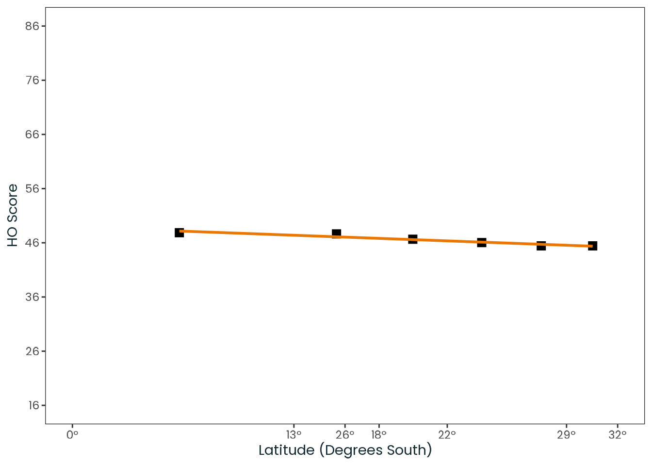
Source: Created by the author, based on a data extracted from Leocadio-Miguel et al. (2017, Figure 2).
With Figure K.6, it becomes clear that the data provided by the authors does not demonstrate a relevant effect size.