Appendix C — Chapter 4 supplemental material

You are reading the work-in-progress of this thesis.

This chapter should be readable but is currently undergoing final polishing.

C.1 Data wrangling

The data wrangling processes were performed using the targets R package. The full pipeline can be seen in the _targets.R file at the root of the research compendium.

library(targets)

data <- 
  targets::tar_read("geocoded_data", store = here::here("_targets")) |>
  dplyr::select(
    age, sex, state, region, latitude, longitude, height, weight, work, study,
    msf_sc, sjl, le_week, 
    ) |>
  tidyr::drop_na(msf_sc, age, sex, latitude)

C.2 Distribution of main variables

source(here::here("R/test_normality.R"))
source(here::here("R/utils.R"))

col <- "age"

stats <- data |> 
  magrittr::extract2(col) |> 
  test_normality(
    name = col, 
    threshold = hms::parse_hms("12:00:00"), 
    remove_outliers = FALSE, 
    iqr_mult = 1.5, 
    log_transform = FALSE,
    density_line = TRUE, 
    text_size = env_vars$base_size,
    print = TRUE
  ) |>
  rutils:::shush()
#> # A tibble: 14 × 2
#>   name    value           
#>   <chr>   <chr>           
#> 1 n       79198           
#> 2 n_rm_na 79198           
#> 3 n_na    0               
#> 4 mean    31.9838074965417
#> 5 var     85.2414919292643
#> 6 sd      9.23263190695179
#> # ℹ 8 more rows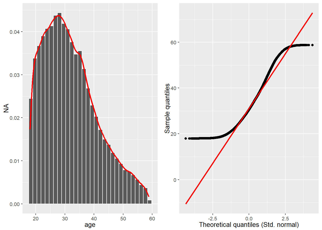

Source: Created by the author.

Figure C.1: Age frequencies among sample subjects.

stats$stats |> list_as_tibble()

name	value
n	79198
n_rm_na	79198
n_na	0
mean	31.9838074965417
var	85.2414919292643
sd	9.23263190695179
min	18
q_1	24.7222222222222
median	30.5388888888889
q_3	37.61875
max	58.7861111111111
iqr	12.8965277777778
skewness	0.665751526654394
kurtosis	2.82381488030798

Source: Created by the author.

Table C.1: Age statistics of sample subjects

C.3 Geographic distribution

source(here::here("R/plot_brazil_uf_map.R"))

rutils:::assert_internet()

brazil_uf_map <- 
  data |> 
  plot_brazil_uf_map(option = "viridis", text_size = env_vars$base_size)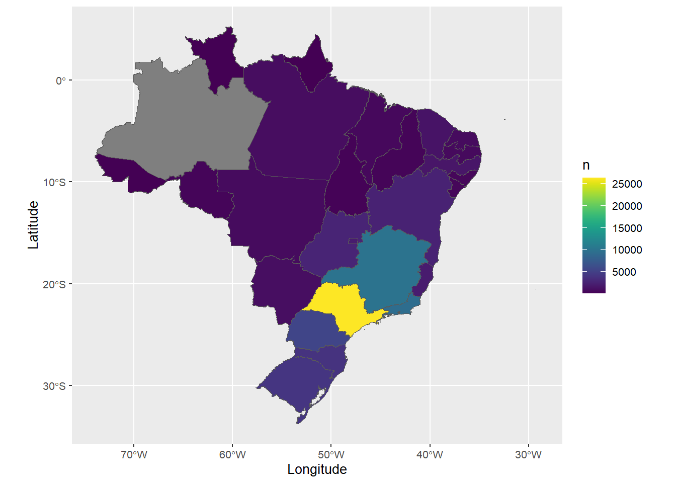

Source: Created by the author.

Figure C.2: Residential geographic distribution among sample subjects

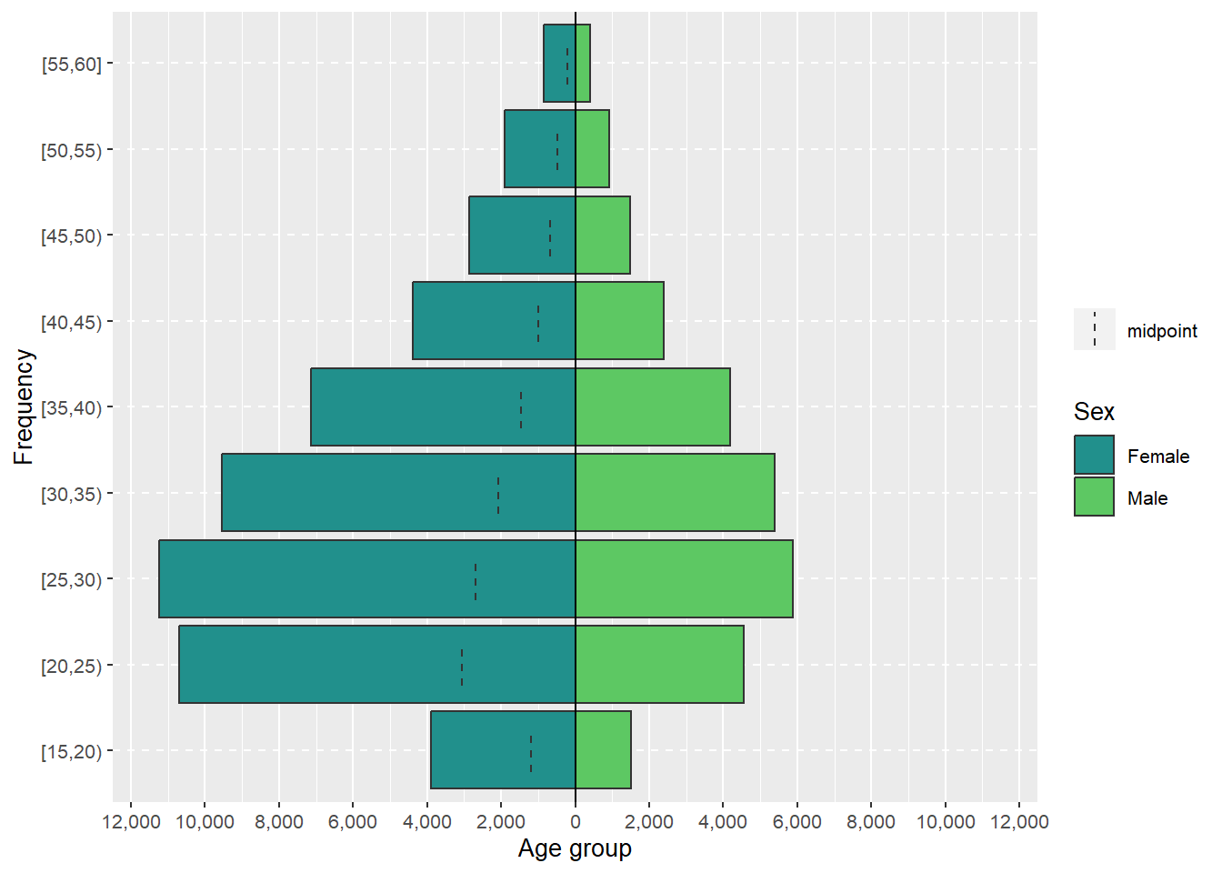
C.4 Age pyramid

source(here::here("R/plot_age_pyramid.R"))

age_pyramid <- 
  data |> 
  plot_age_pyramid(
    interval = 10, 
    na_rm = TRUE, 
    text_size = env_vars$base_size
  )

Source: Created by the author.

Figure C.3: Age pyramid of the sample subjects

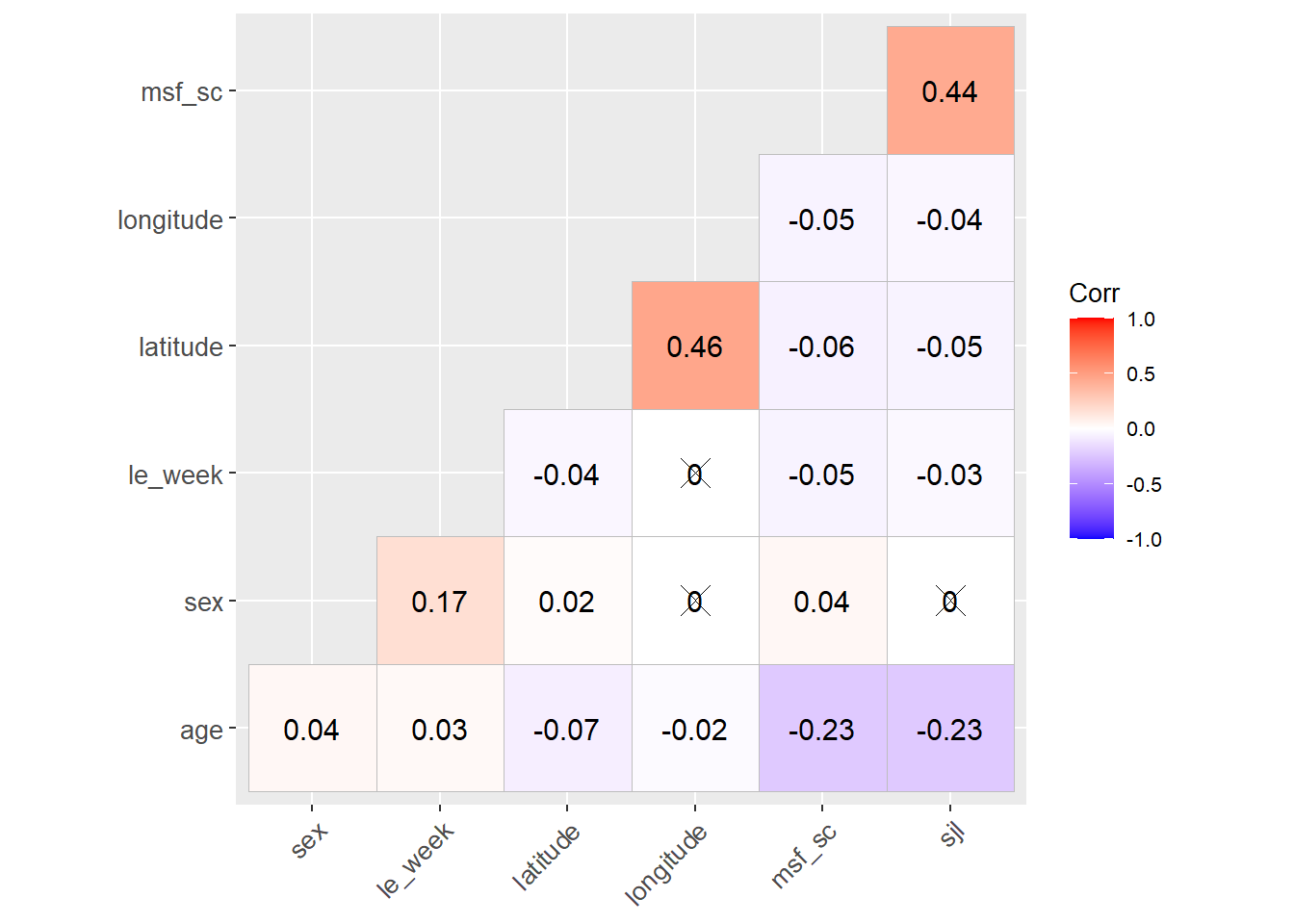
C.5 Correlation matrix

source(here::here("R/plot_ggcorrplot.R"))

cols <- c("sex", "age", "latitude", "longitude", "msf_sc", "sjl", "le_week")

ggcorrplot <-
  data |>
  plot_ggcorrplot(
    cols = cols, 
    na_rm = TRUE, 
    text_size = env_vars$base_size, 
    hc_order = TRUE
    )

Source: Created by the author.

Figure C.4: Correlation matrix of main variables

C.6 Age and sex series

C.6.1 Age/sex versus chronotype

source(here::here("R/plot_age_series.R"))

col <- "msf_sc"
y_lab <- latex2exp::TeX("Local time ($MSF_{sc}$)")

data |>
  dplyr::filter(age <= 50) |>
  plot_age_series(
    col = col, 
    y_lab = y_lab, 
    line_width = 2, 
    boundary = 0.5, 
    point_size = 1,
    error_bar_width = 0.5, 
    error_bar_linewidth = 0.5, 
    error_bar = TRUE,
    text_size = env_vars$base_size
    )

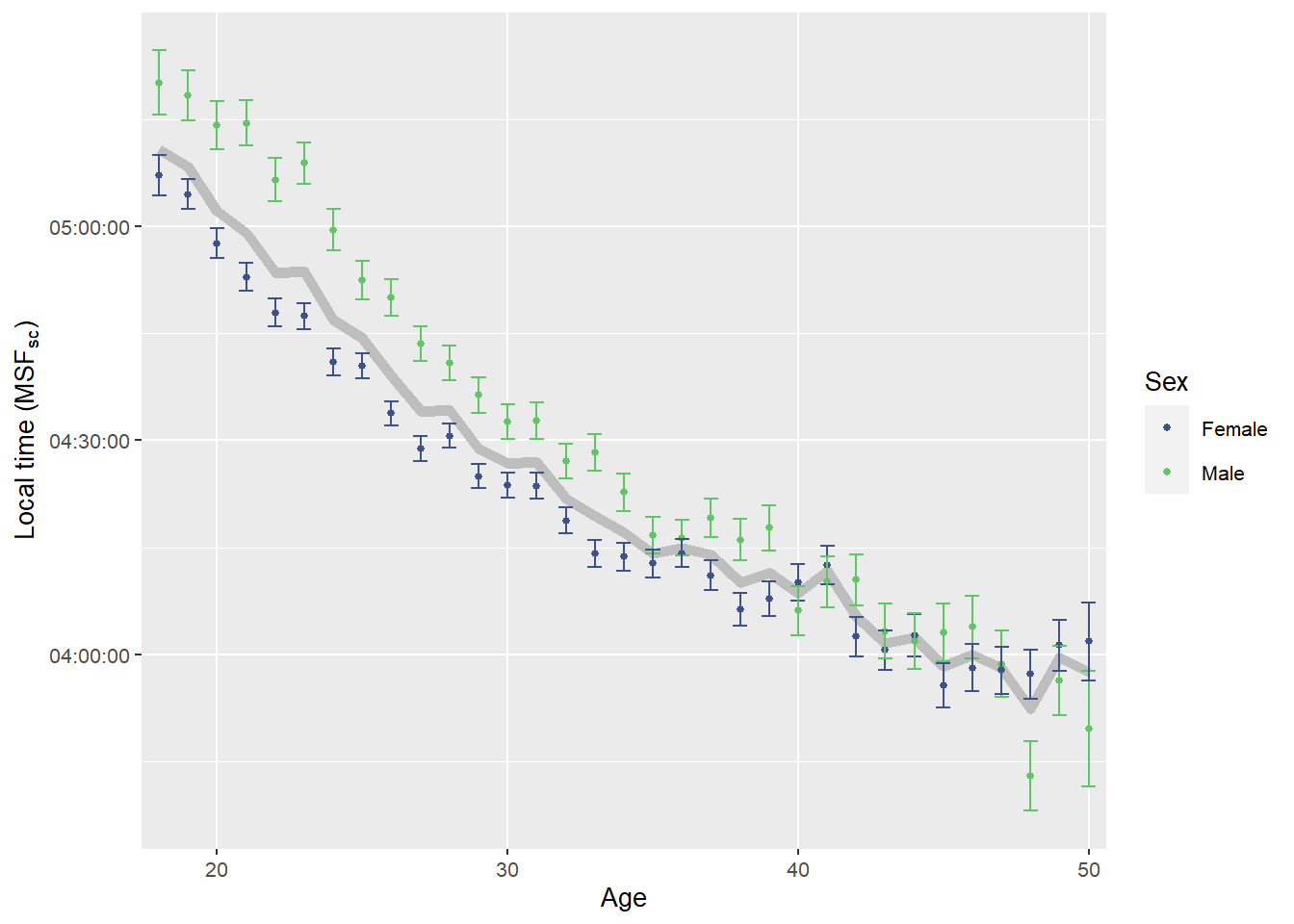
Source: Created by the author. Based on data visualization found in Roenneberg et al. (2007).

Figure C.5: Relation between age and chronotype, divided by sex. Chronotype is represented by the local time of the sleep corrected midpoint between sleep onset and sleep end on work-free days (MSF_sc), MCTQ proxy for measuring the chronotype. The gray line represents both sex. Vertical lines represent the standard error of the mean (SEM).

C.6.2 Age/sex versus weight

source(here::here("R/plot_age_series.R"))

col <- "weight"
y_lab <- "Weight (kg)"

data |>
  dplyr::filter(age <= 50) |>
  plot_age_series(
    col = col, 
    y_lab = y_lab, 
    line_width = 2, 
    boundary = 0.5, 
    point_size = 1,
    error_bar_width = 0.5, 
    error_bar_linewidth = 0.5, 
    error_bar = TRUE,
    text_size = env_vars$base_size
    )

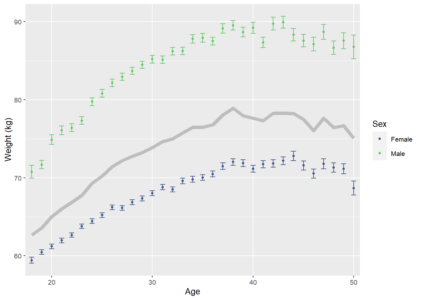
Source: Created by the author. Based on data visualization found in Roenneberg et al. (2007).

Figure C.6: Relation between age and weight (kg), divided by sex. The gray line represents both sex. Vertical lines represent the standard error of the mean (SEM).

C.7 Chronotype distribution

source(here::here("R/plot_chronotype.R"))

col <- "msf_sc"
y_lab <- latex2exp::TeX("Local time ($MSF_{sc}$)")

data |>
  plot_chronotype(
    col = col, 
    x_lab = "Frequency (%)",
    y_lab = y_lab,
    col_width = 0.8, 
    col_border = 0.6, 
    text_size = env_vars$base_size,
    legend_position = "right",
    chronotype_cuts = FALSE
  )

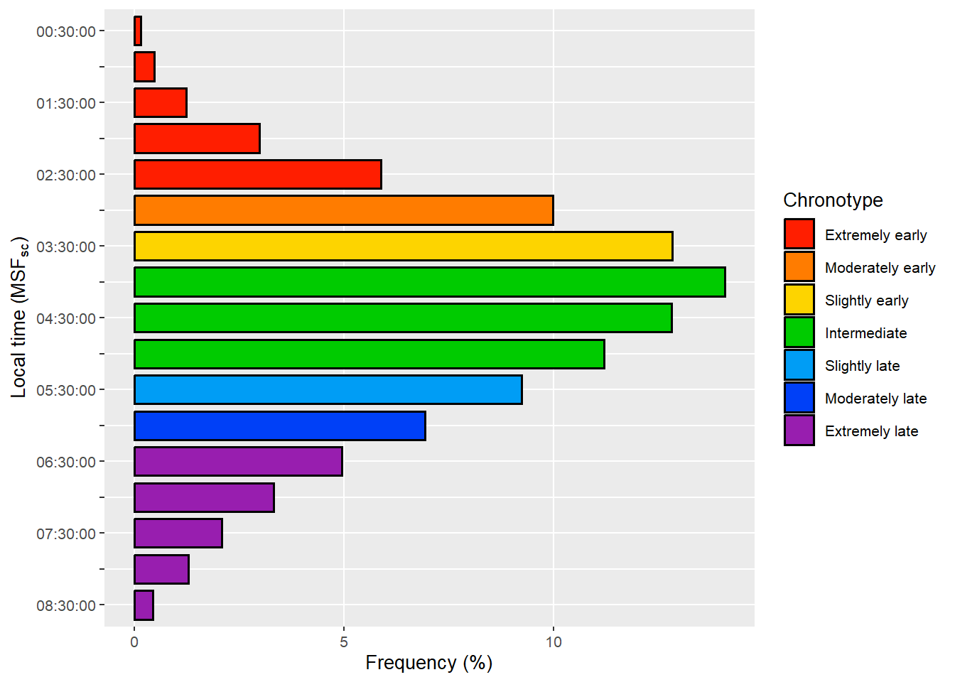
Source: Created by the author. Based on data visualization found in Roenneberg et al. (2019).

Figure C.7: Distribution of the local time of the sleep corrected midpoint between sleep onset and sleep end on work-free days (MSF_sc), MCTQ proxy for measuring the chronotype. The categorical cut-offs follow a quantile approach going from extremely early (\(0 |- 0.11\)) to the extremely late (\(0.88 - 1\)).

C.8 Latitude series

source(here::here("R/plot_latitude_series.R"))

col <- "msf_sc"
y_lab <- latex2exp::TeX("$MSF_{sc} \\pm SEM$")

data |>
  dplyr::filter(age <= 50) |>
  plot_latitude_series(
    col = col, 
    y_lab = y_lab, 
    line_width = 2, 
    point_size = 3,
    error_bar_width = 0.5, 
    error_bar_linewidth = 1, 
    error_bar = TRUE,
    text_size = env_vars$base_size
  )

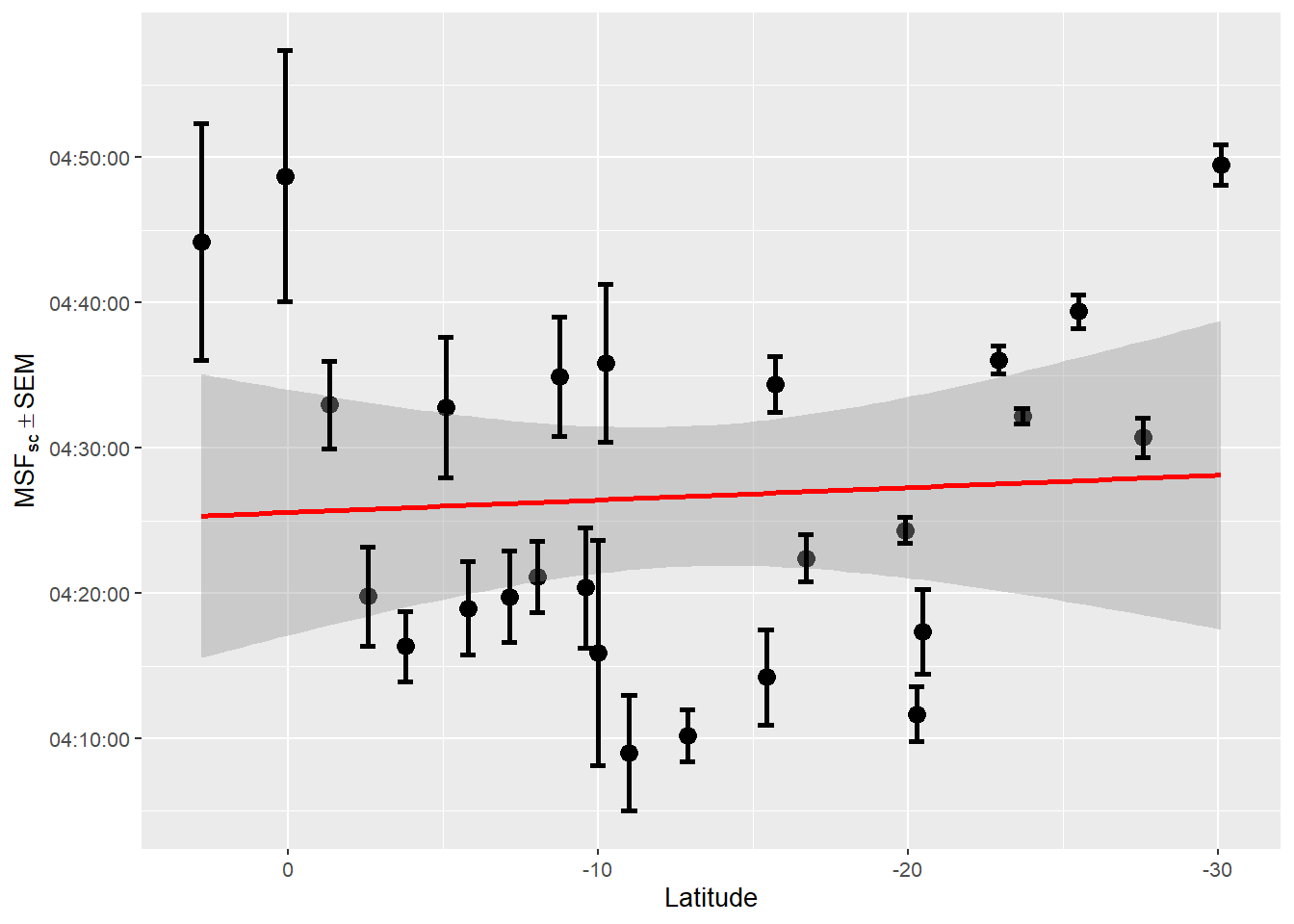
Source: Created by the author. Based on data visualization found in Leocadio-Miguel et al. (2017).

Figure C.8: Distribution of mean aggregates of the local time of the sleep corrected midpoint between sleep onset and sleep end on work-free days (MSF_sc), MCTQ proxy for measuring the chronotype, in relation to latitude decimal degree intervals. Higher values of MSF_sc indicate a tendency toward a late chronotype. The red line represents a linear regression, and the shaded area indicates a pointwise 95% confidence interval.

C.9 Statistics

C.9.1 Numerical variables

source(here::here("R/stats_sum.R"))
source(here::here("R/utils.R"))

col <- "msf_sc"

data |>
  magrittr::extract2(col) |>
  stats_sum(print = FALSE) |>
  list_as_tibble()

name	value
n	79198
n_rm_na	79198
n_na	0
mean	04:28:17.770957
var	08:05:53.49992
sd	01:26:51.406096
min	00:22:30
q_1	03:26:25.714286
median	04:20:42.857143
q_3	05:25:42.857143
max	08:31:04.285714
iqr	01:59:17.142857
skewness	0.284586184927996
kurtosis	2.77321491178072

Source: Created by the author.

Table C.2: Statistics of the local time of the sleep corrected midpoint between sleep onset and sleep end on work-free days (MSF_sc), MCTQ proxy for measuring the chronotype, of sample subjects

C.9.2 Sex

# See <https://sidra.ibge.gov.br> to learn more.

library(magrittr)

rutils:::assert_internet()

# Brazil's 2022 census data
census_data <- 
  sidrar::get_sidra(x = 9514) %>% # Don't change the pipe
  dplyr::filter(
    Sexo %in% c("Homens", "Mulheres", "Total"),
    stringr::str_detect(
      Idade, 
      "^(1[8-9]|[2-9][0-9]) (ano|anos)$|^100 anos ou mais$"
    ),
    .[[17]] == "Total"
    ) |>
  dplyr::transmute(
    sex = dplyr::case_when(
      Sexo == "Homens" ~ "Male",
      Sexo == "Mulheres" ~ "Female",
      Sexo == "Total" ~ "Total"
    ),
    value = Valor
  ) |>
  dplyr::group_by(sex) |>
  dplyr::summarise(n = sum(value)) |>
  dplyr::ungroup()

census_data <- 
  dplyr::bind_rows(
    census_data |>
      dplyr::filter(sex != "Total") |>
      dplyr::mutate(
        n_rel = n / sum(n[sex != "Total"]),
        n_per = round(n_rel * 100, 3)
      ),
    census_data |>
      dplyr::filter(sex == "Total") |>
      dplyr::mutate(n_rel = 1, n_per = 100)
  ) |>
  dplyr::as_tibble() |>
  dplyr::arrange(sex)

count <- data |>
  dplyr::select(sex) |>
  dplyr::group_by(sex) |>
  dplyr::summarise(n = dplyr::n()) |>
  dplyr::ungroup() |>
  dplyr::mutate(
    n_rel = n / sum(n),
    n_per = round(n_rel * 100, 3)
  ) |>
  dplyr::arrange(dplyr::desc(n_rel)) |>
  dplyr::bind_rows(
    dplyr::tibble(
      sex = "Total",
      n = nrow(tidyr::drop_na(data, sex)),
      n_rel = 1, 
      n_per = 100
    )
  )

count <- 
  dplyr::left_join(
    count, census_data, 
    by = "sex", 
    suffix = c("_sample", "_census")
  ) |>
  dplyr::mutate(
    n_rel_diff = n_rel_sample - n_rel_census,
    n_per_diff = n_per_sample - n_per_census
  ) |>
  dplyr::relocate(
    sex, n_sample, n_census, n_rel_sample, n_rel_census, n_rel_diff,
    n_per_sample, n_per_census, n_per_diff
  )

count |> dplyr::select(sex, n_per_sample, n_per_census, n_per_diff)

sex	n_per_sample	n_per_census	n_per_diff
Female	66.243	52.263	13.98
Male	33.757	47.737	-13.98
Total	100.000	100.000	0.00

Source: Created by the author. Based on data from Brazil’s 2022 census (Instituto Brasileiro de Geografia e Estatística (n.d.-b)).

Table C.3: Sex frequencies among sample subjects compared with data from Brazil’s 2022 census

sum(count$n_per_diff)
#> [1] -7.105427e-15

C.9.3 Age and sex

source(here::here("R/stats_sum.R"))
source(here::here("R/utils.R"))

value <- "Male"

data |>
  dplyr::filter(sex == value) |>
  magrittr::extract2("age") |>
  stats_sum(print = FALSE) |>
  list_as_tibble()

name	value
n	26735
n_rm_na	26735
n_na	0
mean	32.4343759740665
var	80.9906211885464
sd	8.99947893983571
min	18
q_1	25.5388888888889
median	31.2583333333333
q_3	37.9319444444444
max	58.7722222222222
iqr	12.3930555555556
skewness	0.617696405622681
kurtosis	2.84390555184727

Source: Created by the author.

Table C.4: Age statistics of male sample subjects.

# See <https://sidra.ibge.gov.br> to learn more.

library(magrittr)

rutils:::assert_internet()

# Brazil's 2022 census data
census_data <- 
  sidrar::get_sidra(x = 9514) %>% # Don't change the pipe
  dplyr::filter(
    Sexo %in% c("Homens", "Mulheres", "Total"),
    stringr::str_detect(
      Idade, 
      "^(1[8-9]|[2-9][0-9]) (ano|anos)$|^100 anos ou mais$"
    ),
    .[[17]] == "Total"
    ) |>
  dplyr::transmute(
    sex = dplyr::case_when(
      Sexo == "Homens" ~ "Male",
      Sexo == "Mulheres" ~ "Female",
      Sexo == "Total" ~ "Total"
    ),
    age = as.numeric(stringr::str_extract(Idade, "\\d+")),
    value = Valor
  ) |>
  dplyr::group_by(sex) |>
  dplyr::summarise(
    mean = stats::weighted.mean(age, value),
    sd = sqrt(Hmisc::wtd.var(age, value))
  ) |> 
  dplyr::ungroup() |>
  dplyr::mutate(
    min = c(18, 18, 18),
    max = c(100, 100, 100)
  ) |>
  dplyr::relocate(sex, mean, sd, min, max) |>
  dplyr::as_tibble()

count <- data |>
  dplyr::select(sex, age) |>
  dplyr::group_by(sex) |>
  dplyr::mutate(sex = as.character(sex)) |>
  dplyr::summarise(
    mean = mean(age, na.rm = TRUE), 
    sd = stats::sd(age, na.rm = TRUE),
    min = min(age, na.rm = TRUE), 
    max = max(age, na.rm = TRUE)
    ) |>
  dplyr::ungroup() |>
  dplyr::bind_rows(
    dplyr::tibble(
      sex = "Total",
      mean = mean(data$age, na.rm = TRUE), 
      sd = stats::sd(data$age, na.rm = TRUE),
      min = min(data$age, na.rm = TRUE), 
      max = max(data$age, na.rm = TRUE)
    )
  )
  
count <- 
  dplyr::left_join(
    count, 
    census_data, 
    by = "sex", 
    suffix = c("_sample", "_census")
  ) |>
  dplyr::mutate(mean_diff = mean_sample - mean_census) |>
  dplyr::relocate(
    sex, mean_sample, mean_census, mean_diff, sd_sample, sd_census, 
    min_sample, min_census, max_sample, max_census
  )

count |> 
  dplyr::select(
    sex, mean_sample, mean_census, mean_diff, sd_sample, sd_census
    )

sex	mean_sample	mean_census	mean_diff	sd_sample	sd_census
Female	31.75420	44.98722	-13.23302	9.340939	17.51132
Male	32.43438	43.49903	-11.06465	8.999479	16.86385
Total	31.98381	44.27680	-12.29299	9.232632	17.22133

Source: Created by the author. Based on data from Brazil’s 2022 census (Instituto Brasileiro de Geografia e Estatística (n.d.-b)).

Table C.5: Mean and standard deviation (\(\text{sd}\)) of sample subjects’ age, divided by sex, compared with data from Brazil’s 2022 census

sum(count$mean_diff)
#> [1] -36.59066

C.9.4 Longitudinal range

C.9.4.1 Sample

source(here::here("R/stats_sum.R"))
source(here::here("R/utils.R"))

stats <- 
  data |>
  magrittr::extract2("longitude") |>
  stats_sum(print = FALSE)

abs(stats$max - stats$min)
#> [1] 33.023
stats |> list_as_tibble()

name	value
n	79198
n_rm_na	79198
n_na	0
mean	-45.9455401815147
var	18.9406905927715
sd	4.35209037047388
min	-67.9869962
q_1	-48.4296364
median	-46.9249578
q_3	-43.7756411
max	-34.9639996
iqr	4.6539953
skewness	0.0156480710174436
kurtosis	5.78918700160139

Source: Created by the author.

Table C.6: Residential longitude statistics of sample subjects

C.9.4.2 Brazil

change_sign <- function(x) x * (-1)

## Ponta do Seixas, PB (7° 09′ 18″ S, 34° 47′ 34″ O)
min <- 
  measurements::conv_unit("34 47 34", from = "deg_min_sec", to = "dec_deg") |>
  as.numeric() |>
  change_sign()

## Nascente do rio Moa, AC (7° 32′ 09″ S, 73° 59′ 26″ O)
max <- 
  measurements::conv_unit("73 59 26", from = "deg_min_sec", to = "dec_deg") |>
  as.numeric() |>
  change_sign()

min
#> [1] -34.79278
max
#> [1] -73.99056
abs(max - min)
#> [1] 39.19778

C.9.5 Latitudinal range

C.9.5.1 Sample

source(here::here("R/stats_sum.R"))
source(here::here("R/utils.R"))

stats <- 
  data |>
  magrittr::extract2("latitude") |>
  stats_sum(print = FALSE)

abs(stats$max - stats$min)
#> [1] 32.91596
stats |> list_as_tibble()

name	value
n	79198
n_rm_na	79198
n_na	0
mean	-20.8338507528991
var	40.2956396934244
sd	6.34788466289554
min	-30.1087672
q_1	-23.6820636
median	-23.6820636
q_3	-19.9026404
max	2.8071961
iqr	3.7794232
skewness	1.40629570823769
kurtosis	4.67433697579443

Source: Created by the author.

Table C.7: Residential latitude statistics of sample subjects

C.9.5.2 Brazil

change_sign <- function(x) x * (-1)

## Arroio Chuí, RS (33° 45′ 07″ S, 53° 23′ 50″ O)
min <- 
  measurements::conv_unit("33 45 07", from = "deg_min_sec", to = "dec_deg") |>
  as.numeric() |>
  change_sign()

## Nascente do rio Ailã, RR (5° 16′ 19″ N, 60° 12′ 45″ O)
max <- 
  measurements::conv_unit("5 16 19", from = "deg_min_sec", to = "dec_deg") |>
  as.numeric()

min
#> [1] -33.75194
max
#> [1] 5.271944
abs(max - min)
#> [1] 39.02389

C.9.6 Region

# See <https://sidra.ibge.gov.br> to learn more.

rutils:::assert_internet()

# Brazil's 2022 census data
census_data <- 
  sidrar::get_sidra(x = 4714, variable = 93, geo = "Region") |>
  dplyr::select(dplyr::all_of(c("Valor", "Grande Região"))) |>
  dplyr::transmute(
    col = `Grande Região`,
    n = Valor,
    n_rel = n / sum(n),
    n_per = round(n_rel * 100, 3)
    ) |>
  dplyr::mutate(
    col = dplyr::case_when(
      col == "Norte" ~ "North",
      col == "Nordeste" ~ "Northeast",
      col == "Centro-Oeste" ~ "Midwest",
      col == "Sudeste" ~ "Southeast",
      col == "Sul" ~ "South"
    )
  ) |>
  dplyr::as_tibble() |>
  dplyr::arrange(dplyr::desc(n_rel))

count <- data |> 
  magrittr::extract2("region") |>
  stats_sum(print = FALSE) |>
  magrittr::extract2("count") |>
  dplyr::mutate(
    n_rel = n / sum(n),
    n_per = round(n_rel * 100, 3)
    ) |>
  dplyr::arrange(dplyr::desc(n_rel))

count <- 
  dplyr::left_join(
    count, census_data, by = "col", suffix = c("_sample", "_census")
  ) |>
  dplyr::mutate(
    n_rel_diff = n_rel_sample - n_rel_census,
    n_per_diff = n_per_sample - n_per_census
  ) |>
  dplyr::relocate(
    col, n_sample, n_census, n_rel_sample, n_rel_census, n_rel_diff,
    n_per_sample, n_per_census, n_per_diff
  )

count |> dplyr::select(col, n_per_sample, n_per_census, n_per_diff)

col	n_per_sample	n_per_census	n_per_diff
Southeast	60.565	41.777	18.788
South	17.122	14.742	2.380
Northeast	11.538	26.914	-15.376
Midwest	8.287	8.021	0.266
North	2.489	8.546	-6.057

Source: Created by the author. Based on data from Brazil’s 2022 census (Instituto Brasileiro de Geografia e Estatística (n.d.-a)).

Table C.8: Residential region frequencies among sample subjects compared with data from Brazil’s 2022 census.

sum(count$n_per_diff)
#> [1] 0.001

C.9.7 State

source(here::here("R/stats_sum.R"))

data |> 
  magrittr::extract2("state") |>
  stats_sum(print = FALSE) |>
  magrittr::extract2("count") |>
  dplyr::mutate(
    n_rel = n / sum(n),
    n_per = round(n_rel * 100, 3)
    ) |>
  dplyr::arrange(dplyr::desc(n_rel))

col	n	n_rel	n_per
São Paulo	26379	0.3330766	33.308
Minas Gerais	10115	0.1277179	12.772
Rio de Janeiro	9381	0.1184500	11.845
Paraná	5517	0.0696609	6.966
Rio Grande do Sul	4097	0.0517311	5.173
Santa Catarina	3946	0.0498245	4.982
Goiás	2674	0.0337635	3.376
Bahia	2522	0.0318442	3.184
Espírito Santo	2091	0.0264022	2.640
Distrito Federal	2087	0.0263517	2.635
Pernambuco	1550	0.0195712	1.957
Ceará	1398	0.0176520	1.765
Mato Grosso do Sul	1014	0.0128034	1.280
Pará	938	0.0118437	1.184
Rio Grande do Norte	789	0.0099624	0.996
Mato Grosso	788	0.0099497	0.995
Paraíba	773	0.0097603	0.976
Maranhão	652	0.0082325	0.823
Sergipe	533	0.0067300	0.673
Alagoas	526	0.0066416	0.664
Rondônia	401	0.0050633	0.506
Piauí	395	0.0049875	0.499
Tocantins	268	0.0033839	0.338
Acre	132	0.0016667	0.167
Roraima	119	0.0015026	0.150
Amapá	113	0.0014268	0.143

Source: Created by the author. Based on data from Brazil’s 2022 census (Instituto Brasileiro de Geografia e Estatística (n.d.-a)).

Table C.9: Residential state frequencies among sample subjects compared with data from Brazil’s 2022 census.

Instituto Brasileiro de Geografia e Estatística. (n.d.-a). Tabela 4714: População Residente, Área territorial e Densidade demográfica [Tabela]. SIDRA. Retrieved November 11, 2023, from https://sidra.ibge.gov.br/Tabela/4714

Instituto Brasileiro de Geografia e Estatística. (n.d.-b). Tabela 9514: População residente, por sexo, idade e forma de declaração da idade [Tabela]. SIDRA. Retrieved November 11, 2023, from https://sidra.ibge.gov.br/tabela/9514

Leocadio-Miguel, M. A., Louzada, F. M., Duarte, L. L., Areas, R. P., Alam, M., Freire, M. V., Fontenele-Araujo, J., Menna-Barreto, L., & Pedrazzoli, M. (2017). Latitudinal cline of chronotype. Scientific Reports, 7(1), 5437. https://doi.org/10.1038/s41598-017-05797-w

Roenneberg, T., Kuehnle, T., Juda, M., Kantermann, T., Allebrandt, K., Gordijn, M., & Merrow, M. (2007). Epidemiology of the human circadian clock. Sleep Medicine Reviews, 11(6), 429–438. https://doi.org/10.1016/j.smrv.2007.07.005

Roenneberg, T., Pilz, L. K., Zerbini, G., & Winnebeck, E. C. (2019). Chronotype and social jetlag: A (self-) critical review. Biology, 8(3), 54. https://doi.org/10.3390/biology8030054