Compute the proportion of time spent in a specific state

state_prop() computes the proportion of time spent in one or more specified states from a tsibble object. It quantifies the fraction of time each day (or epoch) that the subject spends in the target state(s), such as sleeping or awake, across the observed period.

Usage

state_prop(data, state_col = "state", state_values = 1)

Arguments

data: A tsibble object.
state_col: (optional) A string indicating which column of data have the states data (default: "state").
state_values: (optional) An integerish vector indicating which state values are considered as the target state(s) for calculating the proportion (default: 1).

Value

A tsibble object with the following columns:

time: An hms object representing the time of day.
state: A list with a factor of the state at each time point, indicating whether it is the target state or not.
prop: A numeric vector representing the proportion of time spent in the target state at each time point. This value is calculated as the number of occurrences of the target state divided by the total number of observations at that time point.

Examples

library(curl)
library(dplyr)
library(ggplot2)
library(scales)

if (has_internet()) {
  file <- get_from_zenodo(
    doi = "10.5281/zenodo.4898822",
    dir = tempdir(),
    file = "processed.txt"
  )

  data <- read_acttrust(file, tz = "America/Sao_Paulo")
  state_prop_data <- data |> state_prop(state_values = 1) # Sleeping state

  state_prop_data |> print()

  state_prop_data |> pull(prop) |> summary() |> print()

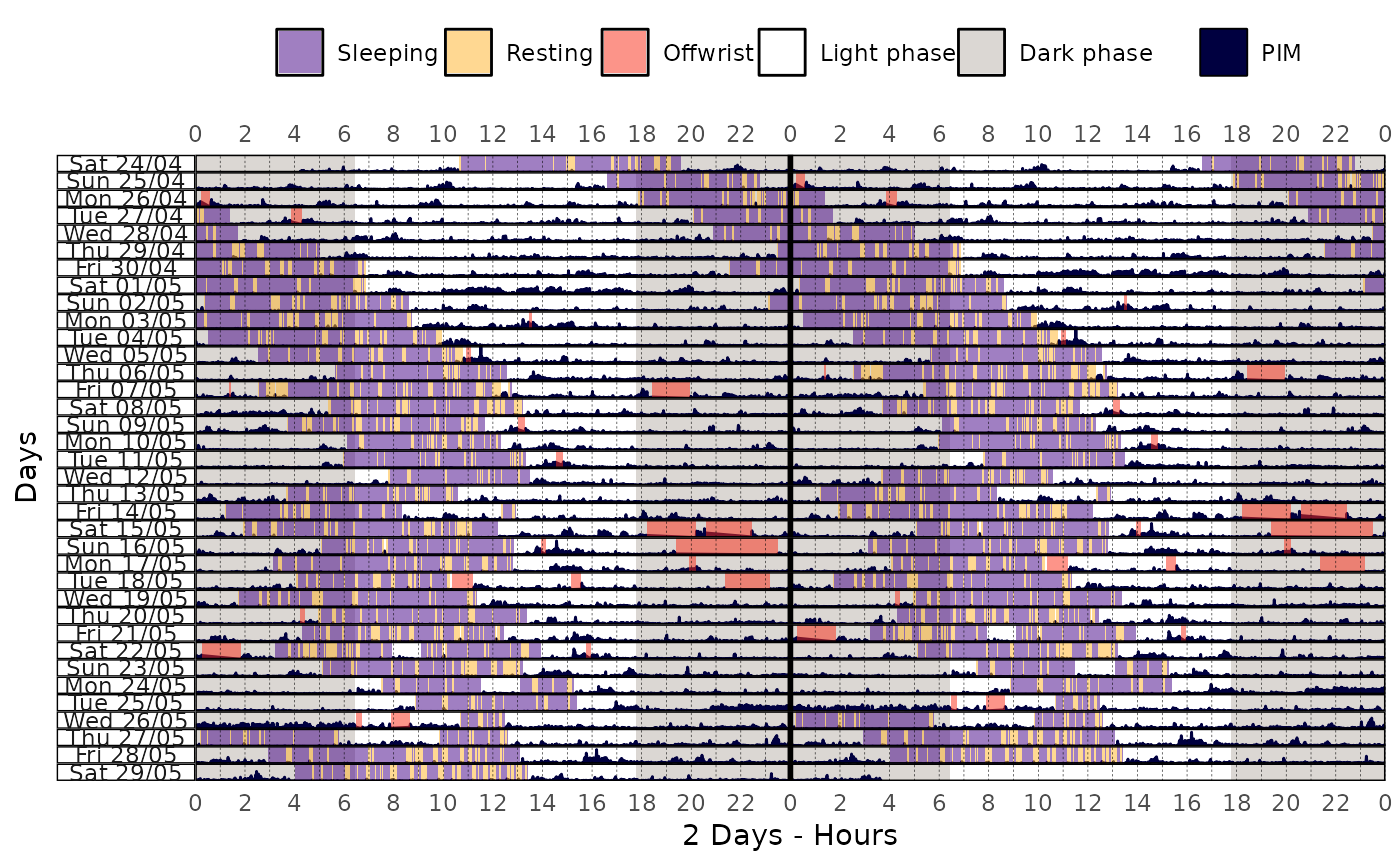
  data |>
    actogram(
      col = "pim",
      days = -1,
      latitude = -23.55065,
      longitude = -46.63338,
      double_plot = TRUE
    )

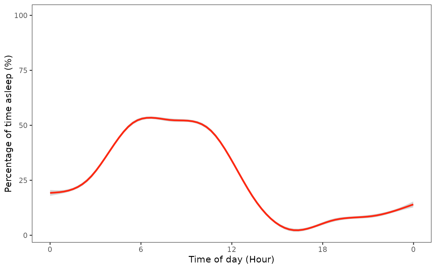
  state_prop_data |>
    mutate(per = prop * 100) |>
    ggplot(ggplot2::aes(x = time, y = per)) +
    geom_smooth(color = "#FC2913") +
    labs(
      x = "Time of day (Hour)",
      y = "Percentage of time asleep (%)",
    ) +
    scale_x_time(
      breaks = breaks_width("6 hours"),
      labels = label_time("%-H") # Use "%#H" for Windows
    ) +
    scale_y_continuous(limits = c(NA, 100)) +
    actverse:::get_actverse_theme()
}
#> ℹ Reading data
#> ✔ Reading data [130ms]
#> 
#> ℹ Tidying data
#> ✔ Tidying data [341ms]
#> 
#> ℹ Validating data
#> ℹ Found 2 gap in the time series: 2021-04-26 03:14:00/2021-04-26 03:14:00 and 2021-05-01 17:34:00/2021-05-01 17:34:00 (showing up to a total of 5 values).
#> ℹ Validating data

#> ℹ Found 21 offwrist blocks in the time series. All values were set as NA.
#> ℹ Validating data

#> ✔ Validating data [19.1s]
#> 
#> # A tsibble: 1,440 x 3 [1m]
#>    time   state       prop
#>    <time> <list>     <dbl>
#>  1 00'00" <fct [36]> 0.167
#>  2 01'00" <fct [36]> 0.167
#>  3 02'00" <fct [36]> 0.167
#>  4 03'00" <fct [36]> 0.167
#>  5 04'00" <fct [36]> 0.167
#>  6 05'00" <fct [36]> 0.139
#>  7 06'00" <fct [36]> 0.139
#>  8 07'00" <fct [36]> 0.139
#>  9 08'00" <fct [36]> 0.139
#> 10 09'00" <fct [36]> 0.167
#> # ℹ 1,430 more rows
#>    Min. 1st Qu.  Median    Mean 3rd Qu.    Max. 
#> 0.00000 0.08333 0.19444 0.25408 0.44444 0.66667 

#> `geom_smooth()` using method = 'gam' and formula = 'y ~ s(x, bs = "cs")'

Compute the proportion of time spent in a specific state

Usage

Arguments

Value

See also

Examples