Compute Phillips et al.'s Sleep Regularity Index (SRI)

sri() computes the Sleep Regularity Index (SRI) as described by Phillips et al. (2017) from a tsibble object, quantifying the consistency of sleep/wake patterns across days.

Usage

sri(data, state_col = "state", sleeping_states = 1, awake_states = c(0, 2))

Arguments

data: A tsibble object.
state_col: (optional) A string indicating which column of data have the states/categories data (default: "state").
sleeping_states: (optional) An integerish vector indicating which state values are considered as sleeping states (default: 1).
awake_states: (optional) An integerish vector indicating which states values are considered as awake states.

Value

A tsibble object with the following columns:

time: An hms object representing the time of day.
state: A list with a factor of the sleep state at each time point ("Sleeping" or "Awake").
previous_state: A list with a factor of the sleep state at the same time on the previous day.
agreement: A list with a logical vector indicating whether the state matches the previous day's state.
sri: A numeric vector representing the Sleep Regularity Index (SRI). See the Details section to learn more about how the SRI is computed.

Details

The Sleep Regularity Index (SRI) is a measure of sleep regularity, which quantifies the consistency of sleep patterns over time. It is calculated by comparing the state of sleep at a given time of day with the state of sleep at the same time on the previous day.

The index is computed as follows:

For each time point, compare the sleep state (Sleeping/Awake) with the state at the same time on the previous day.
Calculate the proportion of time points where the states match (i.e., agreement).
Scale this proportion to a range from -100 to 100: a score of 100 indicates perfectly regular sleep/wake patterns, while a score of 0 indicates completely random patterns.

Note: While SRI values below 0 are theoretically possible (e.g., in cases of highly irregular patterns such as alternating 24-hour periods of sleep and wake), such occurrences are extremely rare in practice.

See Phillips et al. (2017) to learn more about the SRI and its applications in sleep research.

References

Phillips, A. J. K., Clerx, W. M., O’Brien, C. S., Sano, A., Barger, L. K., Picard, R. W., Lockley, S. W., Klerman, E. B., & Czeisler, C. A. (2017). Irregular sleep/wake patterns are associated with poorer academic performance and delayed circadian and sleep/wake timing. Scientific Reports, 7(1), 3216. doi:10.1038/s41598-017-03171-4

Examples

library(curl)
library(dplyr)
#> 
#> Attaching package: ‘dplyr’
#> The following objects are masked from ‘package:stats’:
#> 
#>     filter, lag
#> The following objects are masked from ‘package:base’:
#> 
#>     intersect, setdiff, setequal, union
library(ggplot2)
library(scales)

if (has_internet()) {
  file <- get_from_zenodo(
    doi = "10.5281/zenodo.4898822",
    dir = tempdir(),
    file = "processed.txt"
  )

  data <- read_acttrust(file, tz = "America/Sao_Paulo")
  sri_data <- data |> sri()

  sri_data |> print()

  sri_data |> pull(sri) |> summary() |> print()

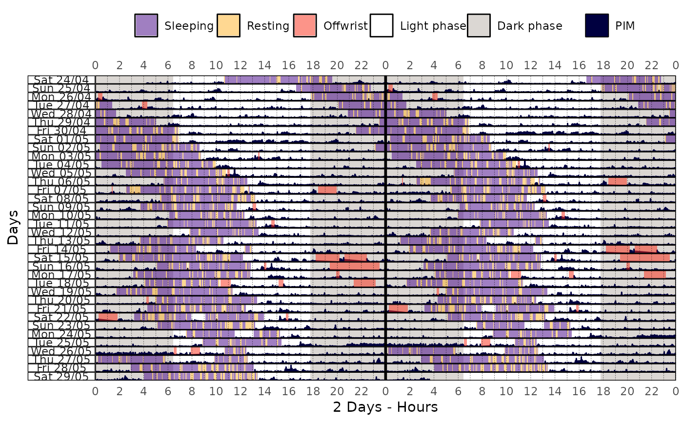
  data |>
    actogram(
      col = "pim",
      days = -1,
      latitude = -23.55065,
      longitude = -46.63338,
      double_plot = TRUE
    )

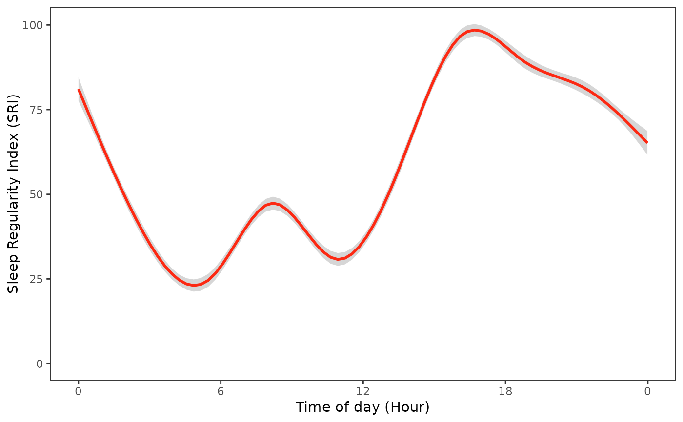
  sri_data |>
    ggplot(ggplot2::aes(x = time, y = sri)) +
    geom_smooth(color = "#FC2913") +
    labs(
      x = "Time of day (Hour)",
      y = "Sleep Regularity Index (SRI)"
    ) +
    scale_x_time(
      breaks = breaks_width("6 hours"),
      labels = label_time("%-H") # Use "%#H" for Windows
    ) +
    scale_y_continuous(limits = c(0, NA)) +
    actverse:::get_actverse_theme()
}
#> ℹ Reading data
#> ✔ Reading data [136ms]
#> 
#> ℹ Tidying data
#> ✔ Tidying data [414ms]
#> 
#> ℹ Validating data
#> ℹ Found 2 gap in the time series: 2021-04-26 03:14:00/2021-04-26 03:14:00 and 2021-05-01 17:34:00/2021-05-01 17:34:00 (showing up to a total of 5 values).
#> ℹ Validating data

#> ℹ Found 21 offwrist blocks in the time series. All values were set as NA.
#> ℹ Validating data

#> ✔ Validating data [17.9s]
#> 
#> # A tsibble: 1,440 x 5 [1m]
#>    time   state      previous_state agreement    sri
#>    <time> <list>     <list>         <list>     <dbl>
#>  1 00'00" <fct [36]> <fct [36]>     <lgl [36]>  77.1
#>  2 01'00" <fct [36]> <fct [36]>     <lgl [36]>  77.1
#>  3 02'00" <fct [36]> <fct [36]>     <lgl [36]>  77.1
#>  4 03'00" <fct [36]> <fct [36]>     <lgl [36]>  77.1
#>  5 04'00" <fct [36]> <fct [36]>     <lgl [36]>  77.1
#>  6 05'00" <fct [36]> <fct [36]>     <lgl [36]>  77.1
#>  7 06'00" <fct [36]> <fct [36]>     <lgl [36]>  77.1
#>  8 07'00" <fct [36]> <fct [36]>     <lgl [36]>  77.1
#>  9 08'00" <fct [36]> <fct [36]>     <lgl [36]>  77.1
#> 10 09'00" <fct [36]> <fct [36]>     <lgl [36]>  77.1
#> # ℹ 1,430 more rows
#>    Min. 1st Qu.  Median    Mean 3rd Qu.    Max. 
#>  -25.00   37.14   63.64   58.78   86.67  100.00 

#> `geom_smooth()` using method = 'gam' and formula = 'y ~ s(x, bs = "cs")'
#> Warning: Removed 21 rows containing non-finite outside the scale range
#> (`stat_smooth()`).