Overview
This vignette will walk you through logolink, an R package that connects R with NetLogo models. By the end, you’ll know how to create experiments, run simulations, and analyze model results, all without ever leaving R.
We’ll work with Wilensky’s Spread of Disease model, an epidemiological simulation based on the SIR equations originally proposed by Kermack and McKendrick (1927). This model is included with NetLogo, so no separate download is required.
This guide assumes familiarity with NetLogo (version 7.0.1 or above) and R programming, particularly the tidyverse ecosystem.
Setting the Stage
You can install logolink like any other R package, using the following command:
install.packages("logolink")logolink do not come with NetLogo, so make sure you have NetLogo installed on your computer. You can download it from the NetLogo website. logolink supports NetLogo version 7.0.1 and above.
After installation, start by loading the package to access its functions:
logolink automatically detects your NetLogo installation path. If automatic detection fails, you can specify it manually. See the run_experiment() documentation for details.
We’ll also need to specify the path to the model file. Since we’re using a built-in NetLogo model, we can retrieve its path easily using the find_netlogo_home() function:
model_path <-
  find_netlogo_home() |>
  file.path(
    "models",
    "IABM Textbook",
    "chapter 6",
    "Spread of Disease.nlogox"
  )
Creating an Experiment
Now that we have our environment set up, let’s start by creating an experiment. We can do this using the create_experiment() function. This function allows us to define the parameters we want to vary, the metrics we want to collect, and other settings for our simulation runs.
setup_file <- create_experiment(
  name = "Population Density (Runtime)",
  repetitions = 10,
  run_metrics_every_step = TRUE,
  time_limit = 1000,
  setup = 'setup',
  go = 'go',
  metrics = 'count turtles with [infected?]',
  constants = list(
    "variant" = "mobile",
    "num-people" = list(
      first = 50,
      step = 50,
      last = 200
    ),
    "connections-per-node" = 4.1,
    "num-infected" = 1,
    "disease-decay" = 0
  )
)
Alternatively, you can define your experiment directly within NetLogo and save it as part of the model file. If you do this, you can skip the create_experiment() step and simply pass the experiment name to run_experiment().
If you’re familiar with the BehaviorSpace XML file structure, you can easily inspect the created experiment using the inspect_experiment() function:
setup_file |> inspect_experiment()
#> <experiments>
#> <experiment name="Population Density (Runtime)" repetitions="10"
#> sequentialRunOrder="true" runMetricsEveryStep="true" timeLimit="1000">
#> <setup>setup</setup>
#> <go>go</go>
#> <metrics>
#> <metric>count turtles with [infected?]</metric>
#> </metrics>
#> <constants>
#> <enumeratedValueSet variable="variant">
#> <value value=""mobile""></value>
#> </enumeratedValueSet>
#> <steppedValueSet variable="num-people" first="50" step="50" last="200">
#> </steppedValueSet>
#> <enumeratedValueSet variable="connections-per-node">
#> <value value="4.1"></value>
#> </enumeratedValueSet>
#> <enumeratedValueSet variable="num-infected">
#> <value value="1"></value>
#> </enumeratedValueSet>
#> <enumeratedValueSet variable="disease-decay">
#> <value value="0"></value>
#> </enumeratedValueSet>
#> </constants>
#> </experiment>
#> </experiments>Running the Simulation
With our experiment defined, we can now run the simulation using the run_experiment(). This function takes care of launching NetLogo, executing the experiment, and collecting the results as tidy data frames.
results <-
  model_path |>
  run_experiment(
    setup_file = setup_file
  )
#> ✔ Running model [4.2s]
#> ✔ Gathering metadata [21ms]
#> ✔ Processing table output [7ms]
Checking the Results
Let’s examine the results.
The output from run_experiment() is a list of data frames. These can be any of the four output formats available in BehaviorSpace: Table, Spreadsheet, Lists, and Statistics. By default, only the Table format is returned, along with some metadata about the experiment run.
The glimpse() function from the dplyr R package can help us take a quick look at the results:
library(dplyr)

results |> glimpse()
#> List of 2
#>  $ metadata:List of 6
#>   ..$ timestamp       : POSIXct[1:1], format: "2026-01-08 03:51:43"
#>   ..$ netlogo_version : chr "7.0.3"
#>   ..$ output_version  : chr "2.0"
#>   ..$ model_file      : chr "Spread of Disease.nlogox"
#>   ..$ experiment_name : chr "Population Density (Runtime)"
#>   ..$ world_dimensions: Named int [1:4] -20 20 -20 20
#>   .. ..- attr(*, "names")= chr [1:4] "min-pxcor" "max-pxcor" ...
#>  $ table   : tibble [8,006 × 8] (S3: tbl_df/tbl/data.frame)
#>   ..$ run_number                 : num [1:8006] 1 1 1 1 1 1 1 1 1 1 ...
#>   ..$ variant                    : chr [1:8006] "mobile" "mobile" ...
#>   ..$ num_people                 : num [1:8006] 50 50 50 50 50 50 ...
#>   ..$ connections_per_node       : num [1:8006] 4.1 4.1 4.1 4.1 ...
#>   ..$ num_infected               : num [1:8006] 1 1 1 1 1 1 1 1 1 1 ...
#>   ..$ disease_decay              : num [1:8006] 0 0 0 0 0 0 0 0 0 0 ...
#>   ..$ step                       : num [1:8006] 0 1 2 3 4 5 6 7 8 9 ...
#>   ..$ count_turtles_with_infected: num [1:8006] 1 1 1 1 1 2 2 2 ...
If you already have an file with BehaviorSpace experiment results, you can read it into R using the read_experiment() function. The output will be the same tidy data frames as those returned by run_experiment().
Analyzing the Data (Bonus Section)
We now have all the data we need to analyze the simulation results, and we did it all without leaving R!
Why stop here, right? Let’s do some basic data wrangling using the dplyr and magrittr packages to prepare the data for analysis and visualization.
library(dplyr)
library(magrittr)

data <-
  results |>
  extract2("table") |>
  rename(infected = count_turtles_with_infected) |>
  mutate(
    variant = as.factor(variant),
    frac_infected = infected / num_people
  ) |>
  summarize(
    mean = mean(frac_infected, na.rm = TRUE),
    sd = sd(frac_infected, na.rm = TRUE),
    .by = c(num_people, step)
  ) |>
  arrange(num_people, step)
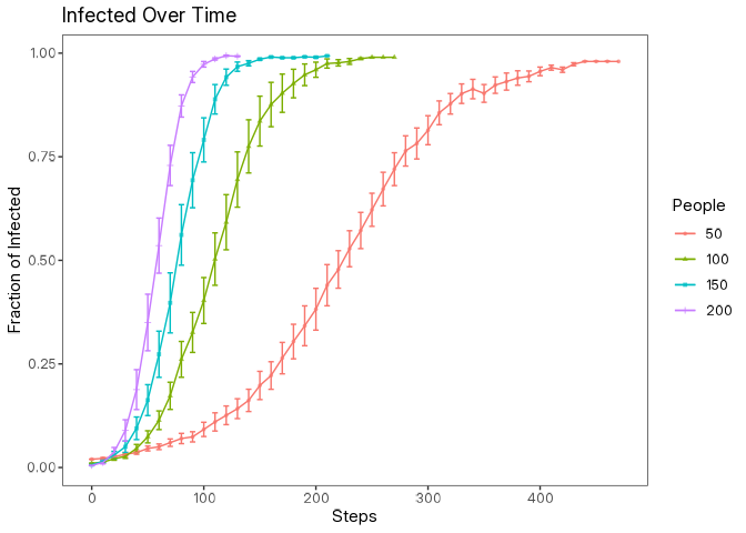
data |> glimpse()Now we can create a simple plot using the ggplot2 package to visualize how the fraction of infected individuals changes over time for different population sizes along with error bars representing the standard error.
library(ggplot2)

data |>
  filter(step %% 10 == 0) |>
  mutate(se = sd / sqrt(10)) |>
  ggplot(aes(
    x = step,
    y = mean,
    color = as.factor(num_people)
  )) +
  geom_point(
    aes(shape = as.factor(num_people)),
    size = 1,
    alpha = 0.75
  ) +
  geom_errorbar(
    aes(
      ymin = mean + se,
      ymax = mean - se
    ),
    width = 5
  ) +
  geom_line() +
  scale_x_continuous(
    breaks = seq(0, max(data$step), 100)
  ) +
  labs(
    title = "Infected Over Time",
    x = "Steps",
    y = "Fraction of Infected",
    color = "People",
    shape = "People"
  )
Visualizing the NetLogo World (Bonus Section)
logolink also allows you to capture screenshots of the NetLogo world during the simulation runs. This is particularly useful for producing publication-quality figures or presentations.
See the Visualizing the NetLogo World tutorial to learn how to do this by using parse_netlogo_color() and get_netlogo_shape() functions.
You can customize these snapshots and animations as needed. Below is an example of an animation using Wilensky’s Wolf Sheep Simple model.
Wrapping up
You now have a basic understanding of how to use logolink to run NetLogo experiments from R. This opens up a world of possibilities for integrating agent-based modeling with statistical analysis and data visualization workflows.
Click here to explore the full list of functions available in logolink.