Filter points on land

filter_points() filters latitude/longitude points that intersects with a given sf geometry.

Note: This function requires the sf package to be installed.

Usage

filter_points(data, geometry)

Arguments

data

A tibble containing the data points to filter. Must include latitude and longitude columns.

geometry

An sf object with the geometry to be used for filtering.

Value

A tibble with the filtered data points.

Examples

# Set the Environment -----

library(curl)
library(dplyr)
library(ggplot2)
library(geobr)
library(sf)
#> Linking to GEOS 3.12.1, GDAL 3.8.4, PROJ 9.4.0; sf_use_s2() is TRUE

plot_geometry <- function(geometry) {
  plot <-
    geometry |>
    ggplot() +
    geom_sf(
      color = "gray75",
      fill = "white",
      inherit.aes = FALSE
    ) +
    labs(x = "Longitude", y = "Latitude")

  print(plot)
}

plot_points <- function(data, geometry) {
  plot <-
    data |>
    ggplot(aes(x = longitude, y = latitude)) +
    geom_sf(
      data = geometry,
      color = "gray75",
      fill = "white",
      inherit.aes = FALSE
    ) +
    geom_point(color = "#3243A6") +
    labs(x = "Longitude", y = "Latitude")

  print(plot)
}

# Define the Points -----

# \dontrun{
  if (has_internet() && test_geobr_connection()) {
    data <- tibble(
      latitude = brazil_state_latitude(),
      longitude = brazil_state_longitude()
    )

    data
  }
#> # A tibble: 27 × 2
#>   latitude longitude
#>      <dbl>     <dbl>
#> 1  -9.98       -67.8
#> 2  -9.65       -35.7
#> 3   0.0402     -51.1
#> 4  -3.13       -60.0
#> 5 -13.0        -38.5
#> 6  -3.73       -38.5
#> # ℹ 21 more rows
# }

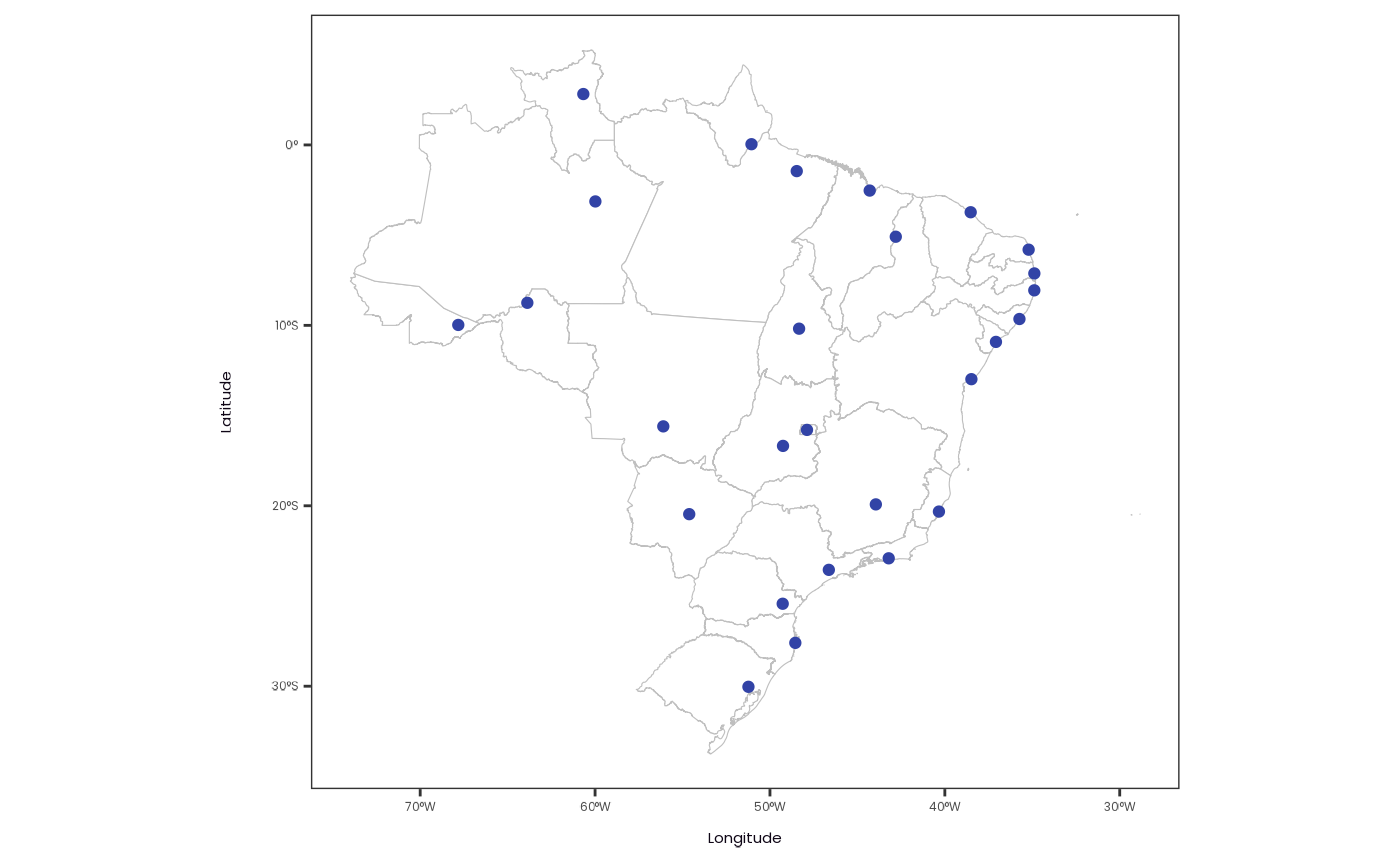
# Visualize the Points on a Map -----

# \dontrun{
  if (has_internet() && test_geobr_connection()) {
    brazil_states_geometry <- read_state()

    data |> plot_points(brazil_states_geometry)
  }
#> Using year/date 2010

# }

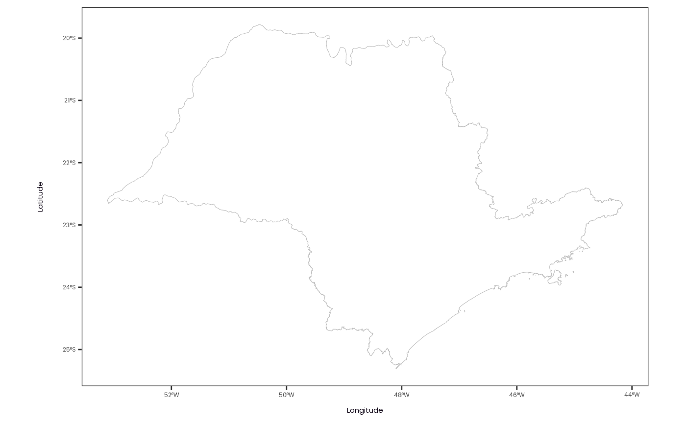
# Set the Geometry to Filter the Points -----

# \dontrun{
  if (has_internet() && test_geobr_connection()) {
    sp_state_geometry <- read_state(code = "SP")

    sp_state_geometry |> plot_geometry()
  }
#> Using year/date 2010

# }

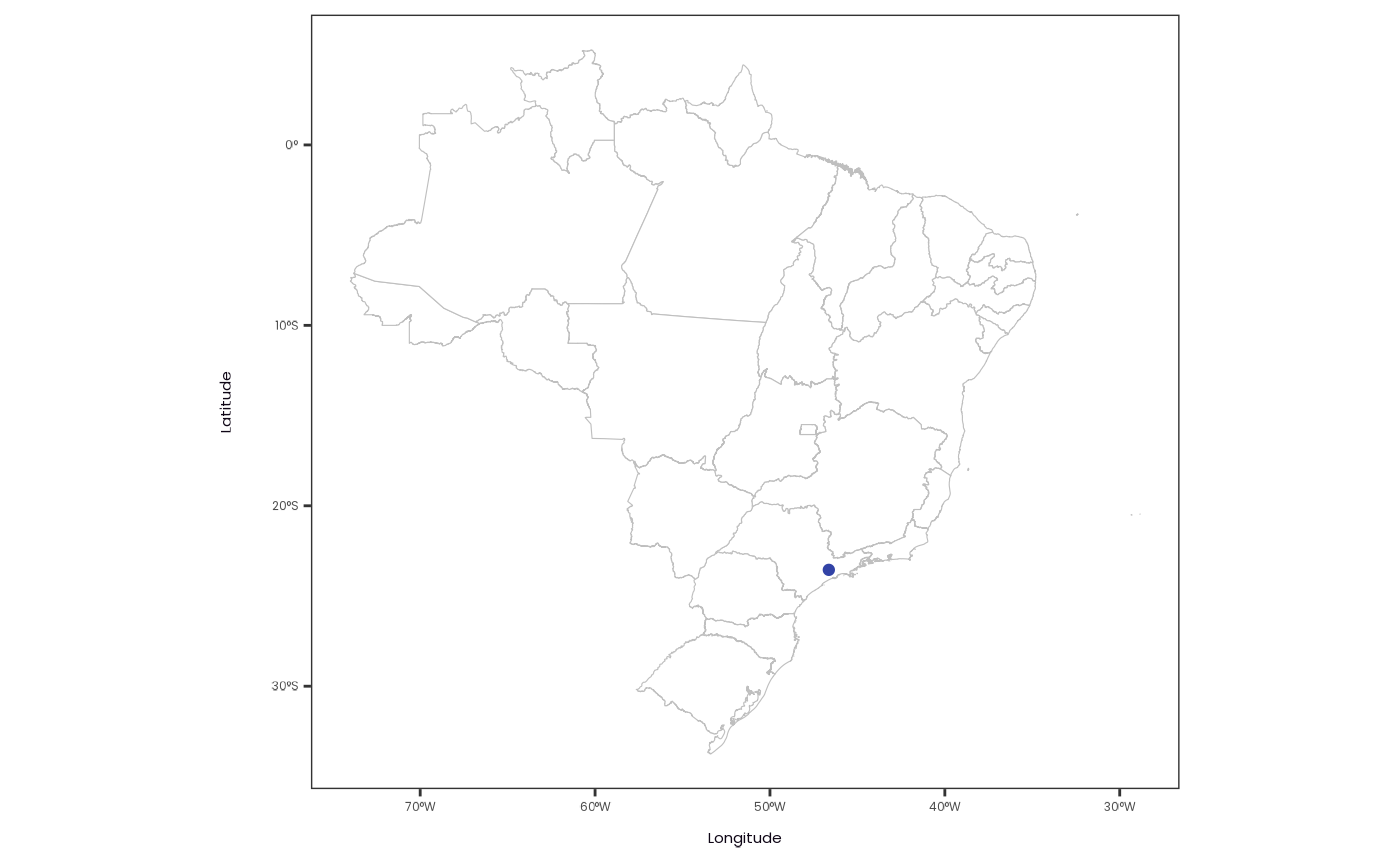
# Filter the Points -----

# \dontrun{
  data <- data |> filter_points(sp_state_geometry)

  data
#> # A tibble: 1 × 2
#>   latitude longitude
#>      <dbl>     <dbl>
#> 1    -23.6     -46.6
# }

# Visualize the Filtered Points -----

# \dontrun{
  data |> plot_points(brazil_states_geometry)

# }