
Is Latitude Associated with Chronotype?
University of São Paulo
2025-02-03
Hi there! 👋
This presentation will provide an overview of the thesis objectives, main concepts, methods, and results. Together, we’ll uncover how environment factors can influence the chronotype.
Here are the main topics:
- Introduction
- Methods
- Results
- Discussion
- Conclusion

Chronotype
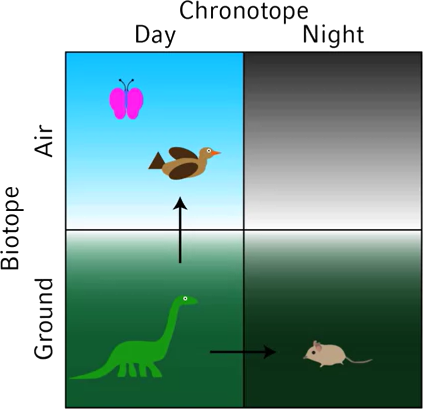
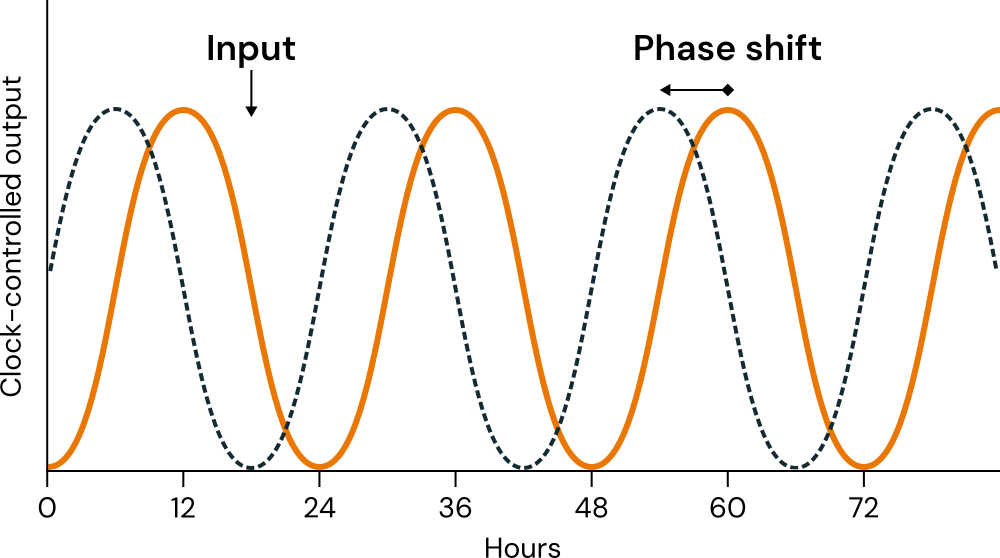
Entrainment
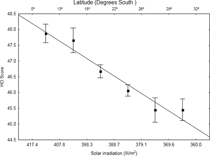
The Latitude Hypothesis

Leocadio-Miguel et al.
Sample: \(12,884\) Brazilian participants.
Method: HO Questionnaire (Horne & Östberg, 1976).
\(\Delta \ \text{Adjusted} \ \text{R}^{2} = 0.388\%\) (Cohen’s \(f^2 = 0.00414\)).
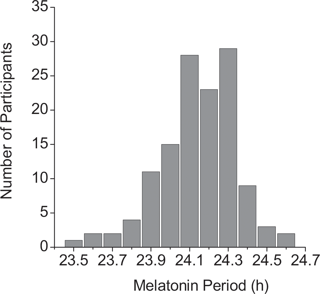
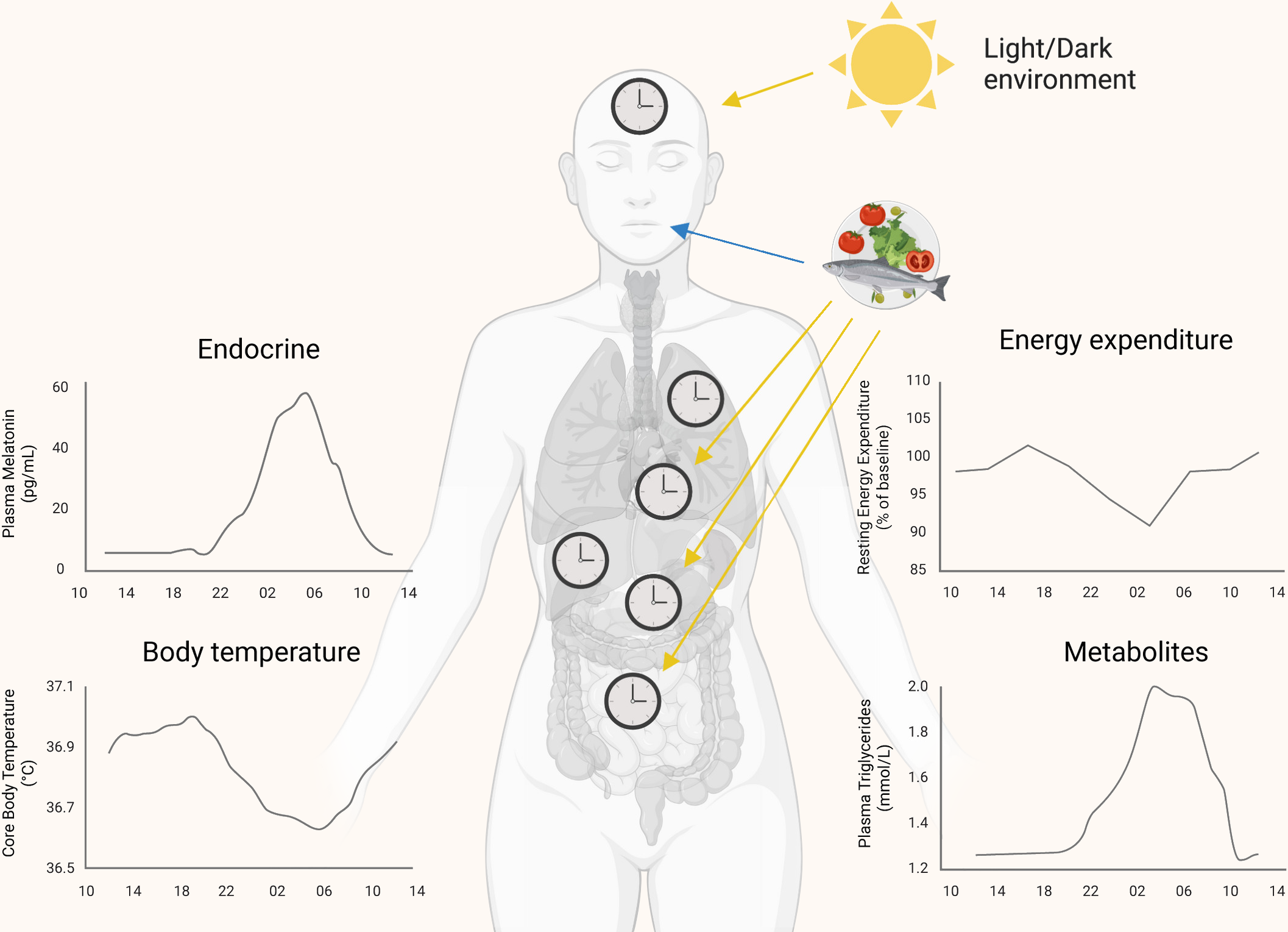
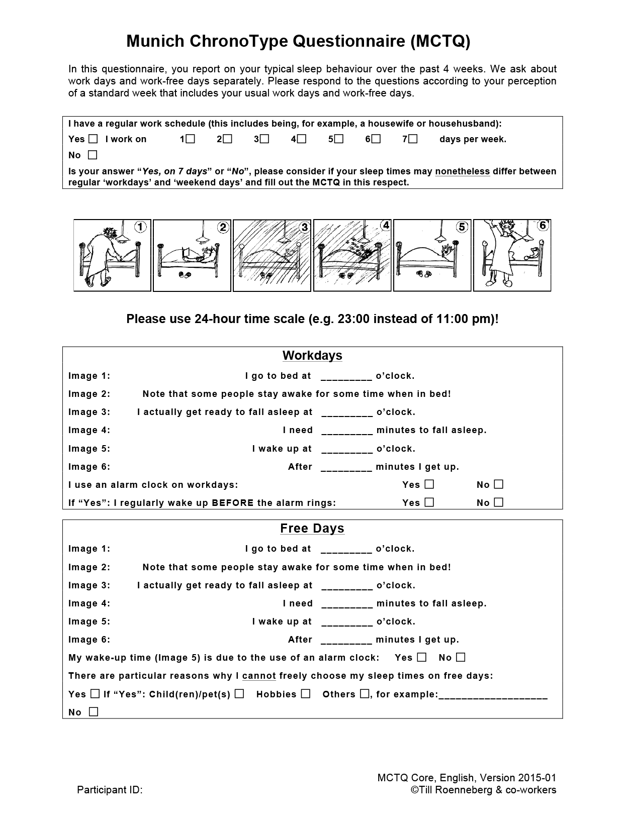
MCTQ
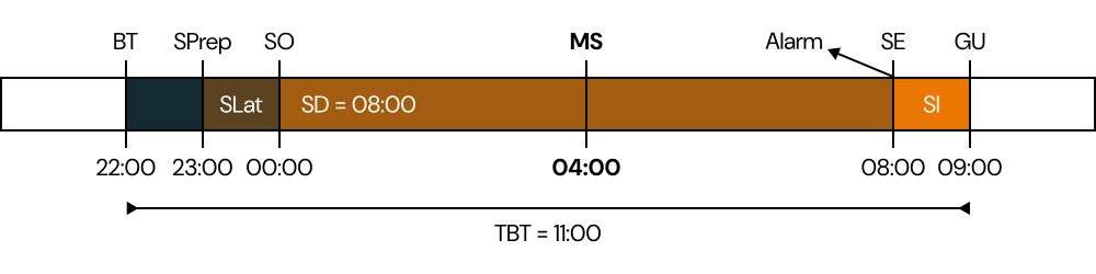
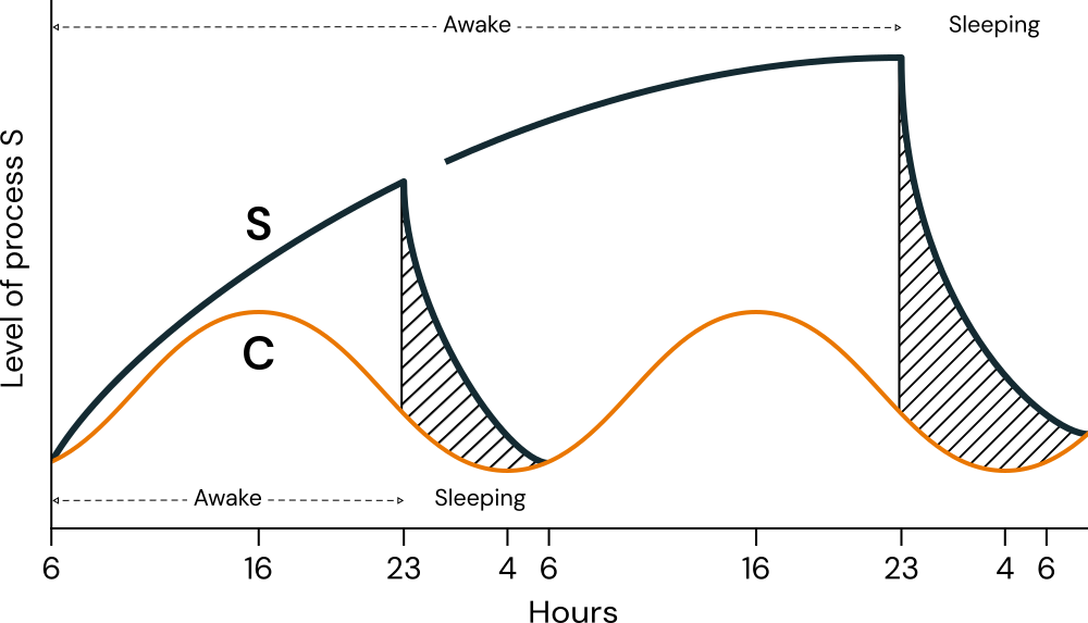
The Two Process of Sleep Reg.
Sample
Sample
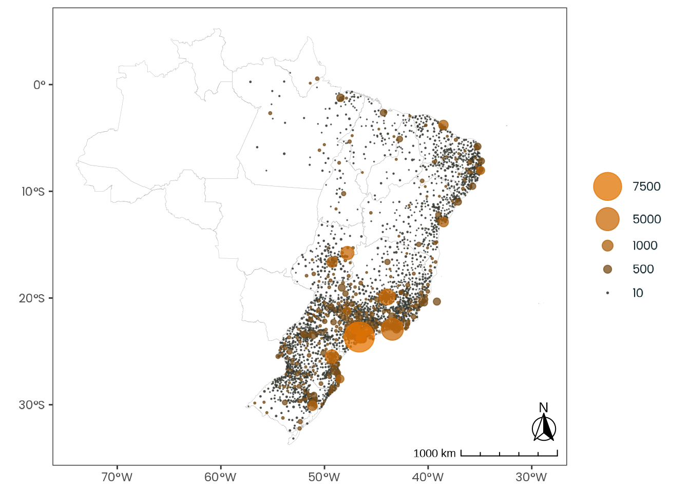
The dataset used for analysis is made up of \(65,824\) Brazilian individuals aged 18 or older, residing in the UTC-3 timezone, who completed the survey between October 15th and 21st, 2017.
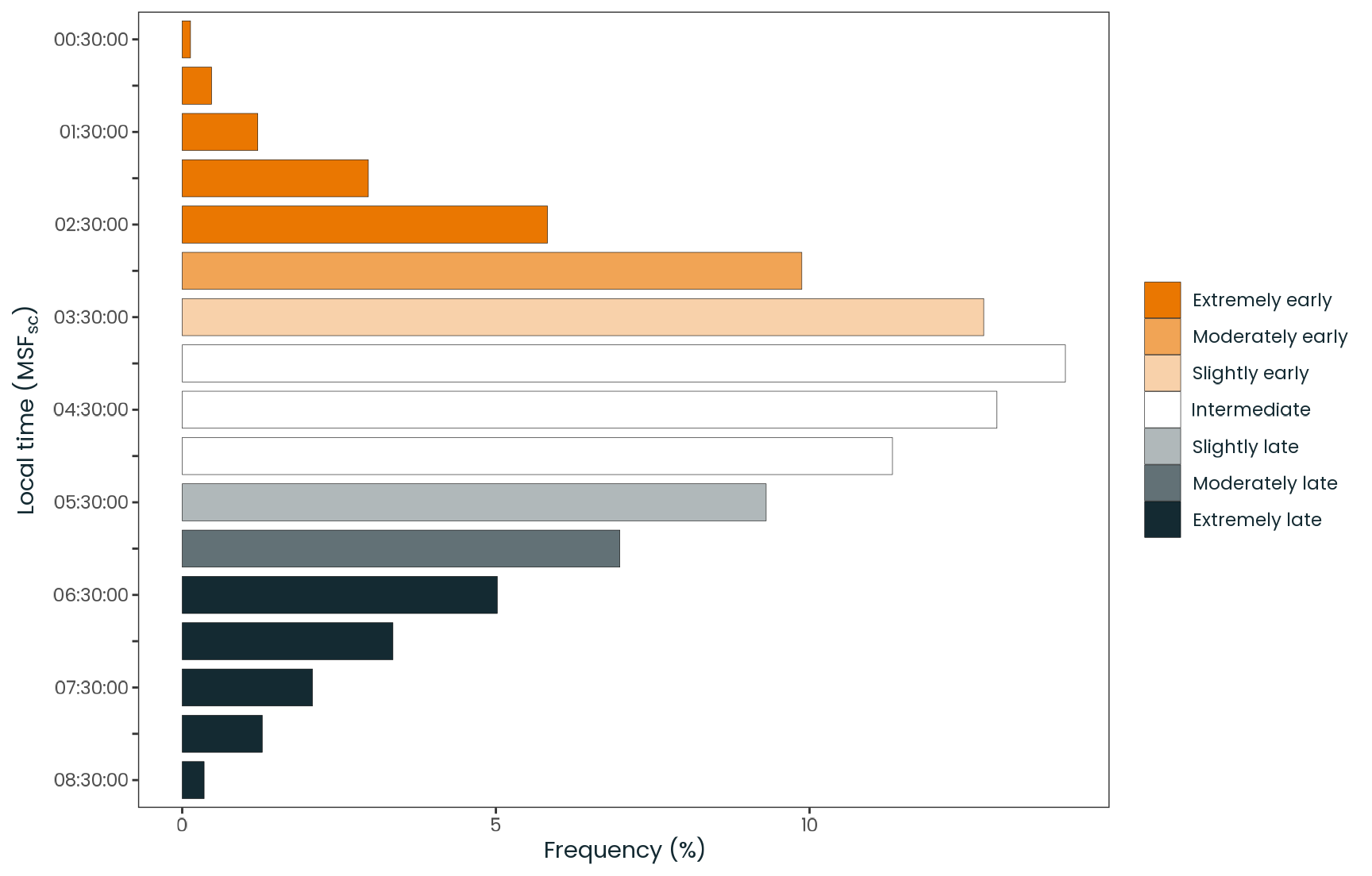
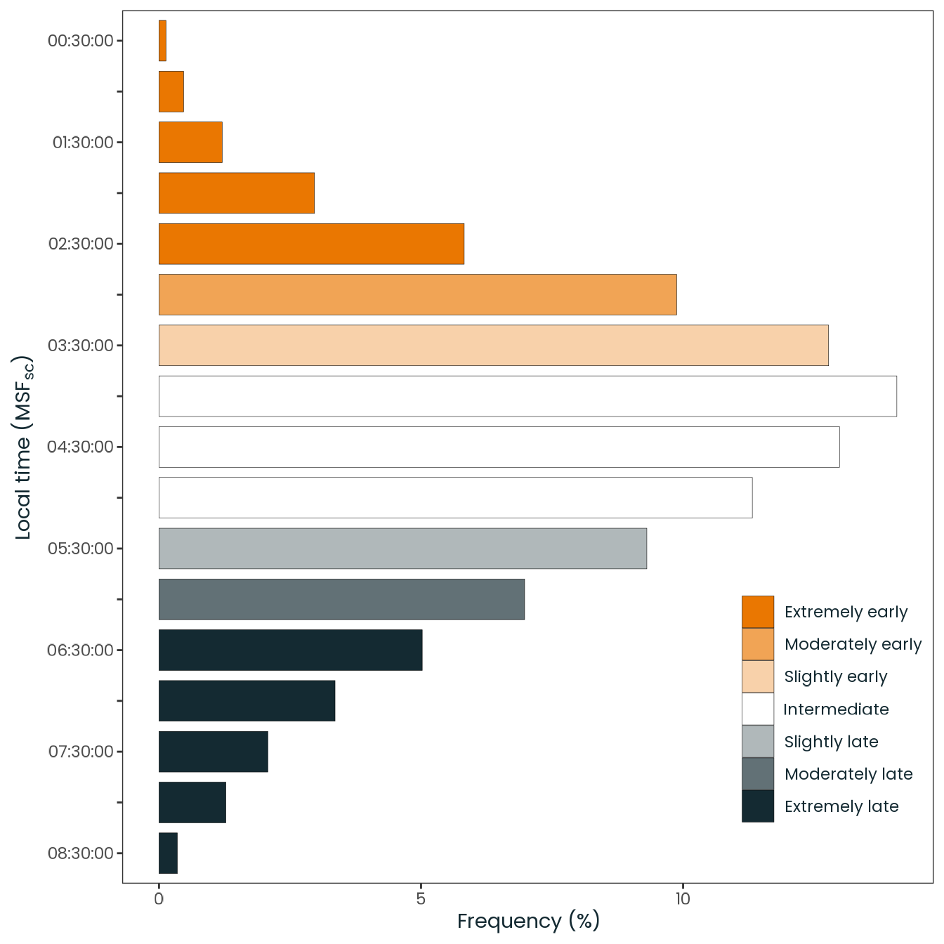
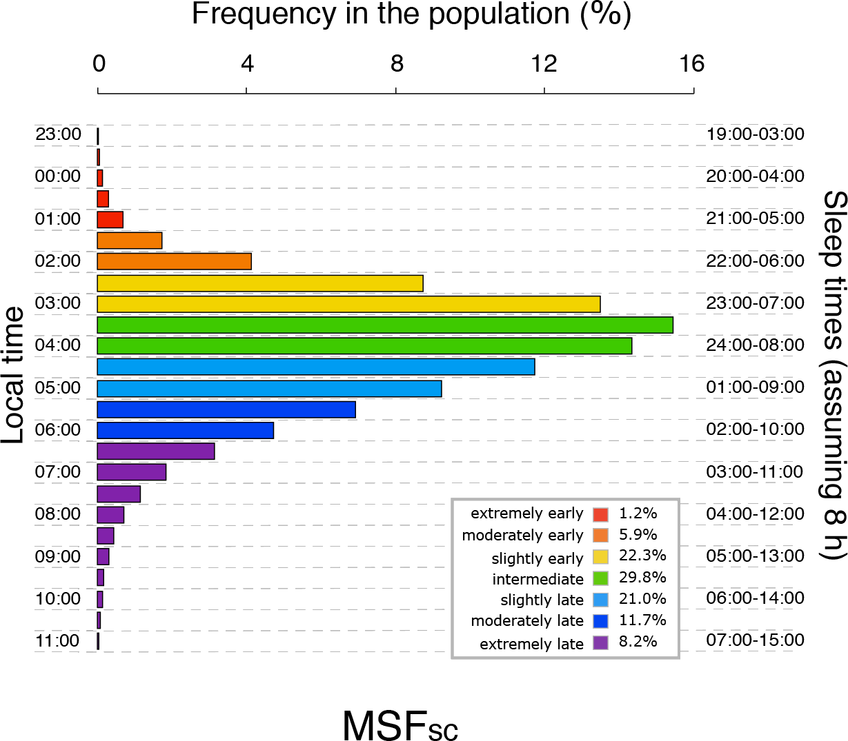
Chronotype Distribution
Hypothesis Test
Restricted Model
(Based on Leocadio-Miguel et al. (2017))
- Predictors (\(4\)):
Age, Sex, Longitude, and the Average Monthly Global Horizontal Irradiance (GHI) at the time of questionnaire completion. - \(\text{R}^2_{\text{adj}} = 0.08517\)
- \(\text{F}(4, 65818) = 1531.829\)
- \(p\text{-value} < 1e-05\)
Chronotype versus Latitude

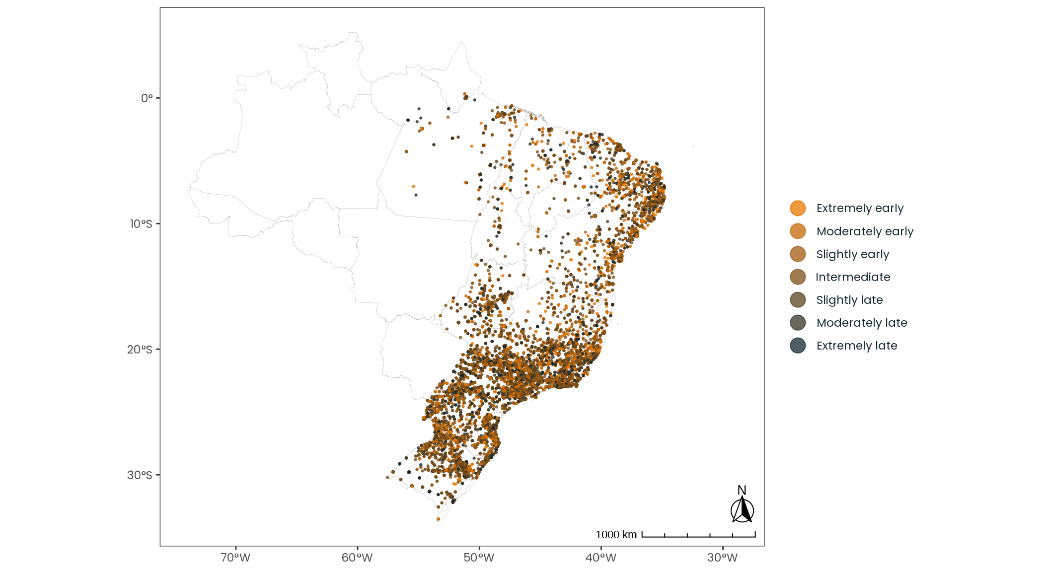
Chronotype Geo. Distribution
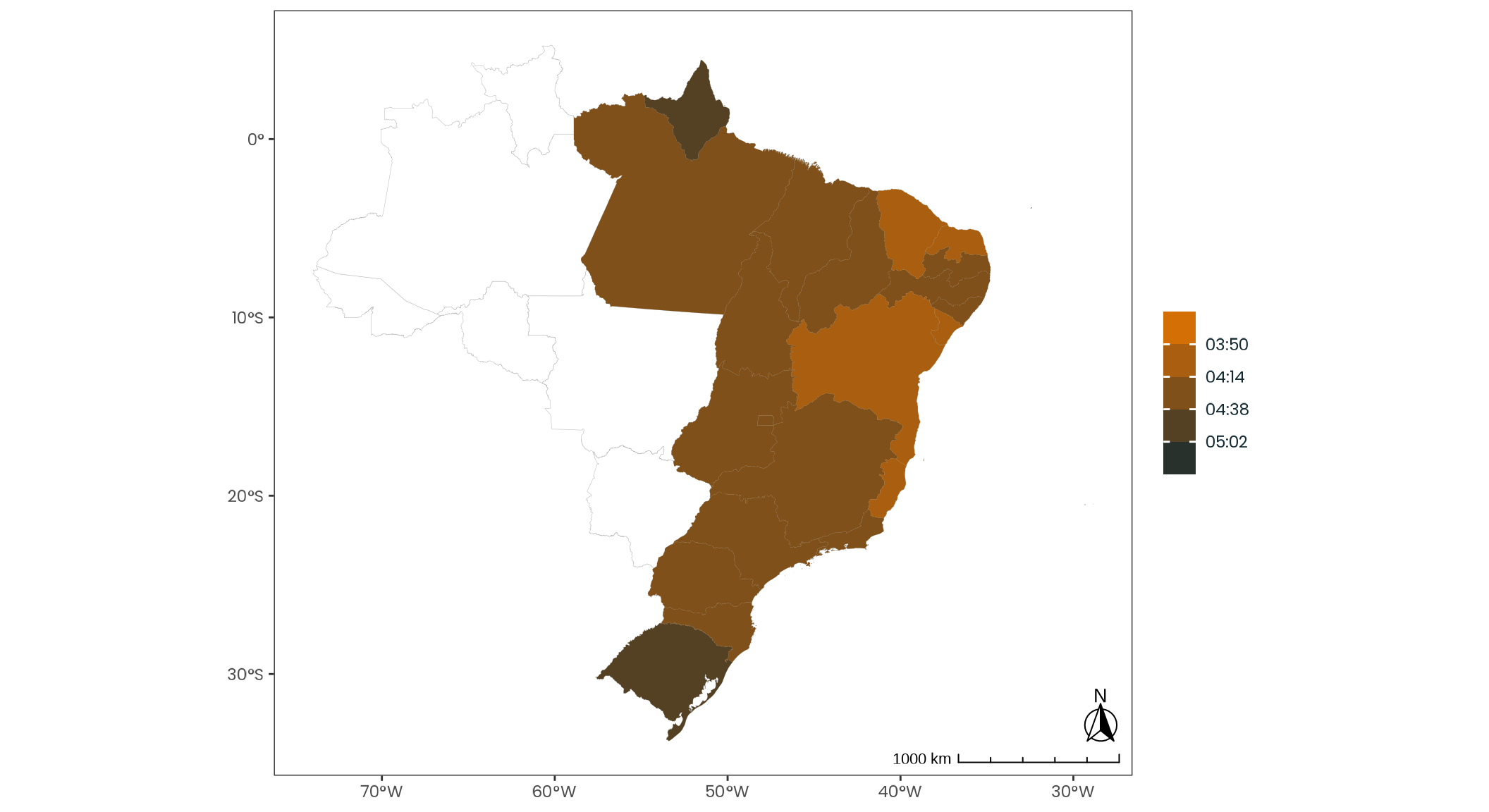
Chronotype Geo. Distribution

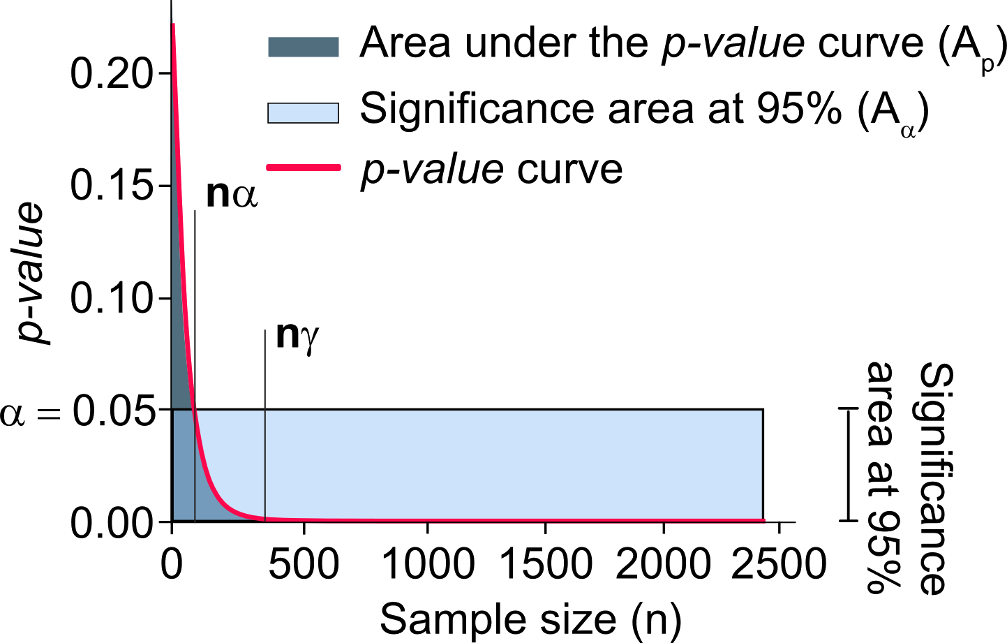
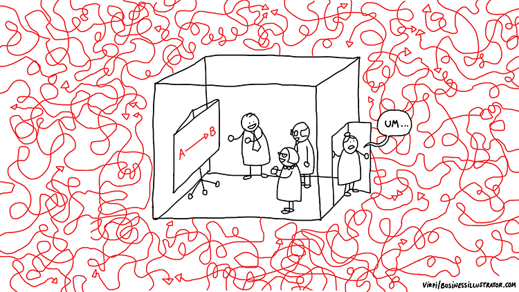
The \(p\)-value Problem
Large samples and sensitivity.
Is a difference of \(0.00001\) valid?
Statistical ritual versus Statistical thinking.
Confirmation bias.
Comparison of a 95% of confidence level (\(\alpha = 0.05\)) and an n-dependent \(p\)-value curve. The parameter \(n_{\alpha}\) represents the minimum sample size to detect statistically significant differences among compared groups. The parameter \(n_{\gamma}\) represents the convergence point of the \(p\)-value curve. When the \(p\)-value curve expresses practical differences, the area under the red curve (\(A_{p(n)}\)) is smaller than the area under the constant function \(\alpha = 0.05\) (\(A_{\alpha = 0.05}\)) when it is evaluated between \(0\) and \(n_{\gamma}\).
The \(p\)-value Problem
SMALL EFFECT SIZE: \(f^2 = .02\). Translated into \(\text{R}^{2}\) or partial \(\text{R}^{2}\) for Case 1, this gives \(.02 / (1 + .02) = .0196\). We thus define a small effect as one that accounts for 2% of the \(\text{Y}\) variance (in contrast with 1% for \(r\)), and translate to an \(\text{R} = \sqrt{0196} = .14\) (compared to .10 for \(r\)). This is a modest enough amount, just barely escaping triviality and (alas!) all too frequently in practice represents the true order of magnitude of the effect being tested. (p. 413)
[…] in many circumstances, all that is intended by “proving” the null hypothesis is that the ES [Effect Size] is not necessarily zero but small enough to be negligible […]. (p. 461)
Nonrealistic Models
Answer
I suggest that it is the aim of science to find satisfactory explanations, of whatever strikes us as being in need of explanation.
This study, using what is arguably one of the largest datasets on chronotype, found no evidence supporting the latitude hypothesis in humans.
Closing remarks
![]()
![]()
This thesis was presented to the School of Arts, Sciences and Humanities (EACH) at the University of São Paulo (USP) as a requirement for the degree of Master of Science by the Graduate Program in Complex Systems Modeling (PPGSCX).
I am deeply grateful to my advisor, Prof. Dr. Camilo Rodrigues Neto, for introducing me to complexity science in 2012, guiding my dissertation with patience, and demonstrating remarkable integrity in navigating a challenging supervisory transition.
Closing remarks
![]()
![]()
The presentation was created using the Quarto publishing system. All analyses presented are fully reproducible and were conducted using the R programming language.
To explore the code and repository for this thesis, click here. The research compendium is also accessible via The Open Science Framework by clicking here.
Financial support was provided by the Coordination for the Improvement of Higher Education Personnel (CAPES) (Grant number: 88887.703720/2022-00).
(AP) Mimosa Pudica
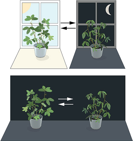
(AP) Entrainment
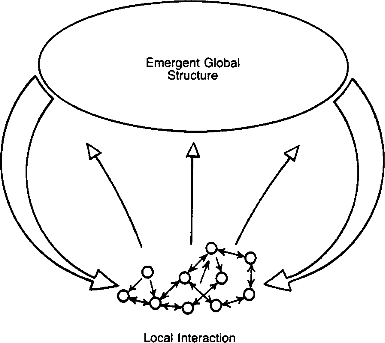
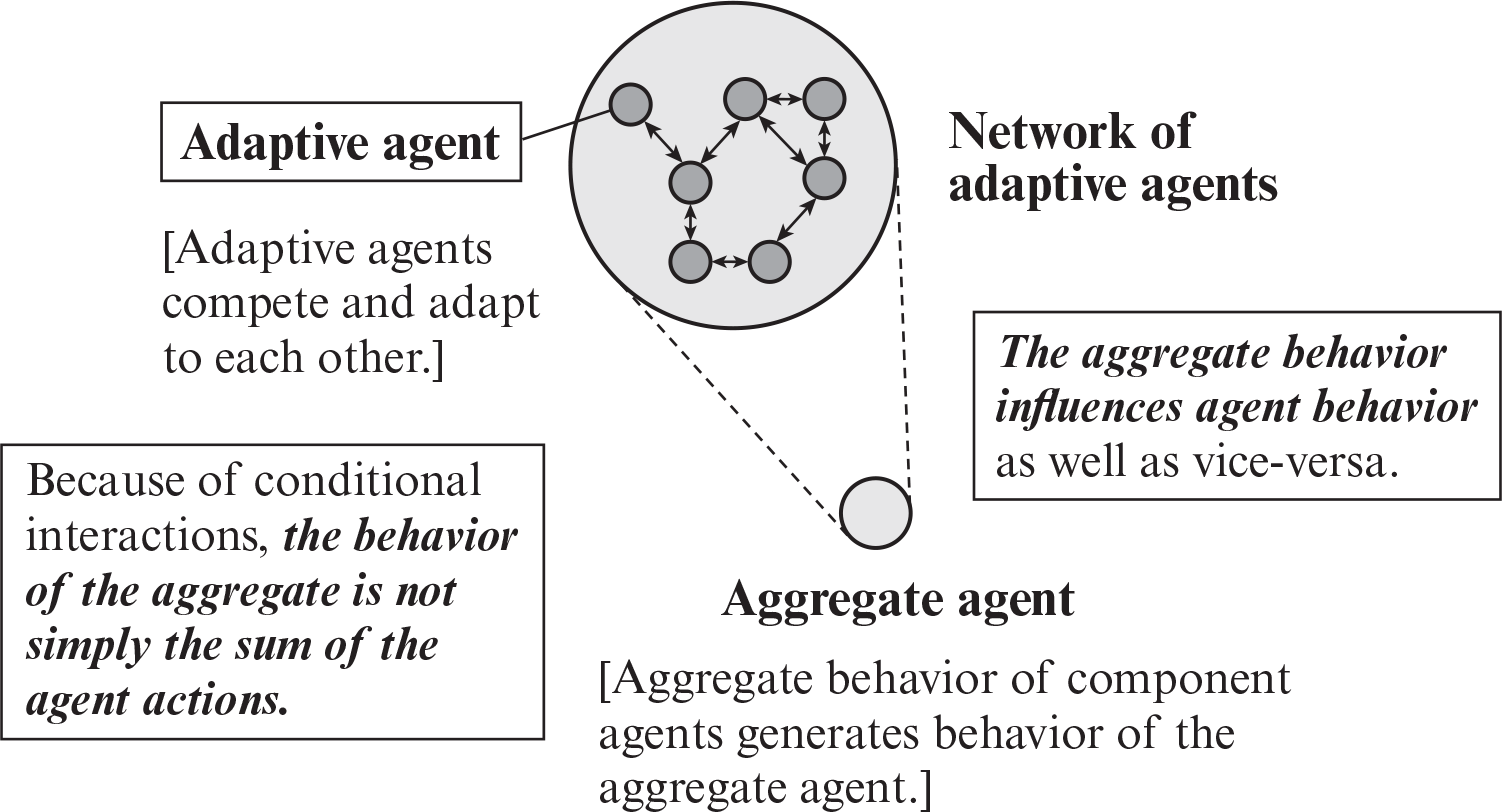
(AP) Emergence
Stable macroscopic patterns arising from local interaction of agents (Epstein, 1999).
When the aggregate exhibits properties not attained by summation (Holland, 2014).


(AP) Emergence
(AP) Emergence
An aggregate behavior emerges from the interactions of the parts (CAS) (Holland, 2012).
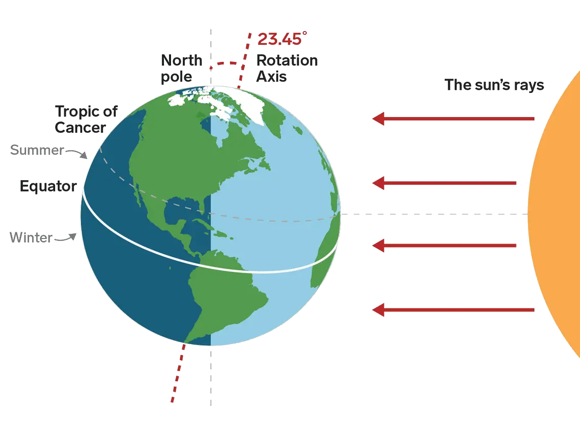
(AP) Earth’s Rotation Axis
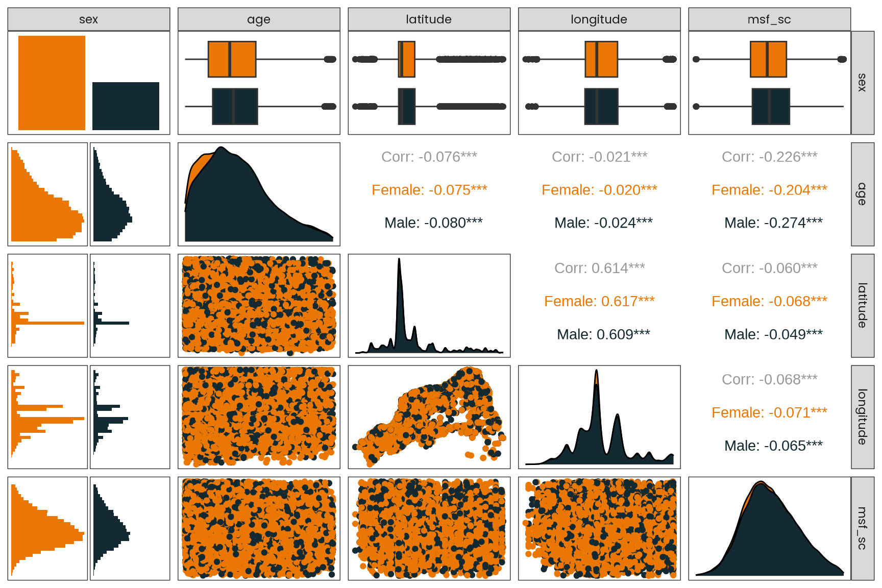
(AP) Corr. Matrix
(AP) Chronotype Comparison
Brazil
Europe
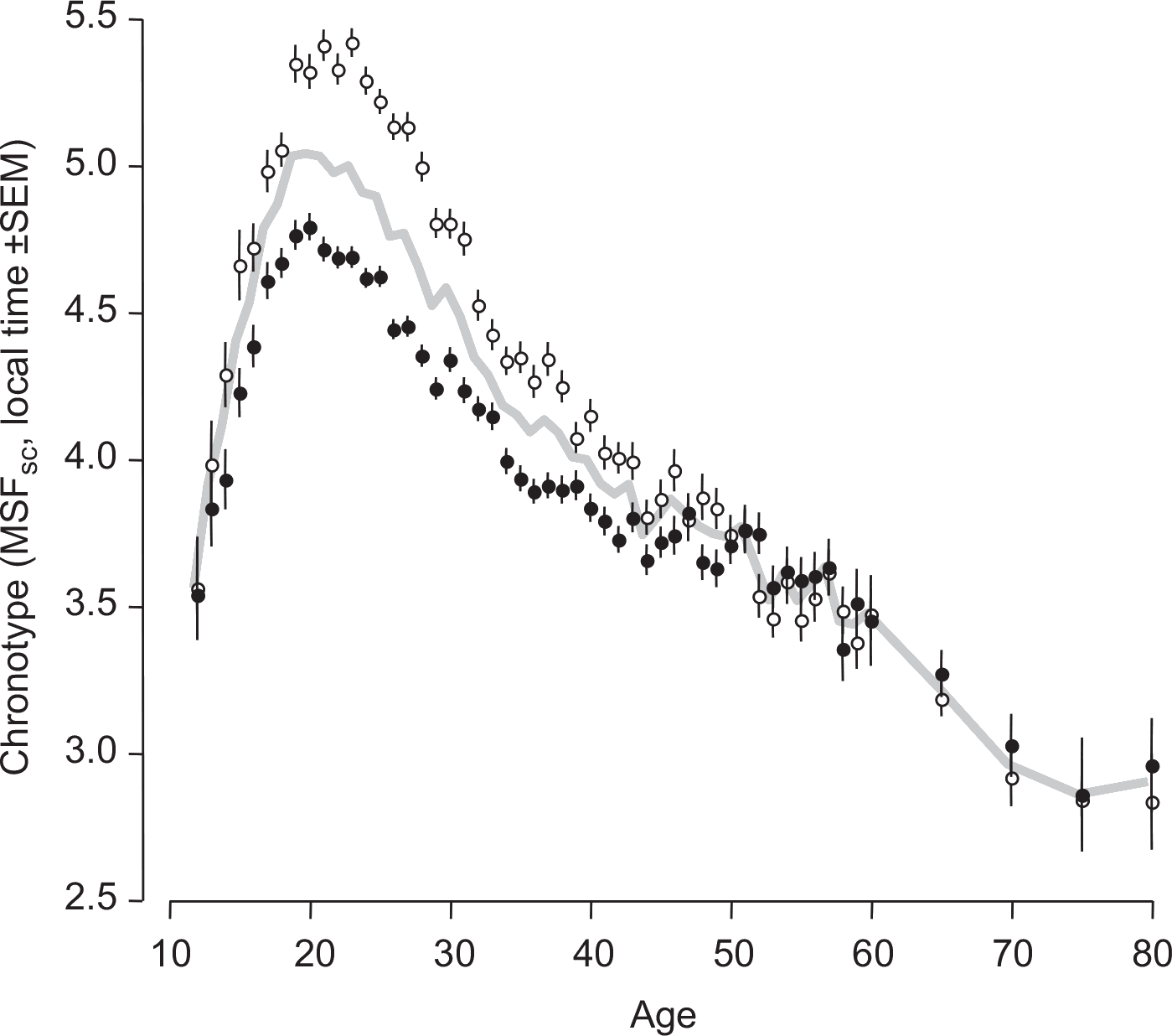
(AP) Age versus Chronotype
Brazil
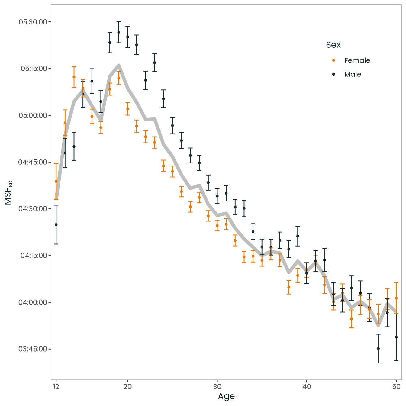
Europe
(AP) Chronotype Geo. Dist.
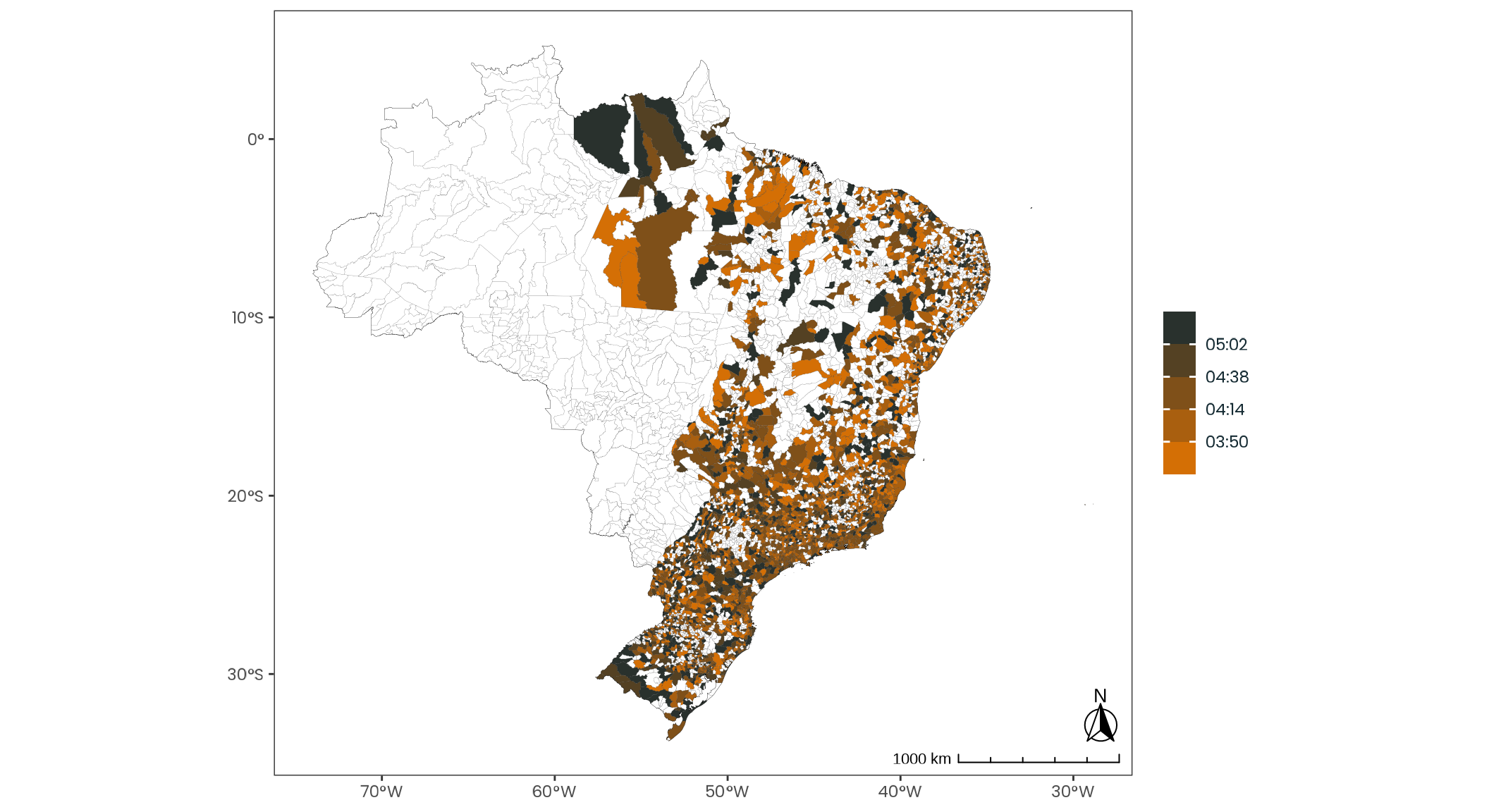
(AP) Chronotype Geo. Dist.
(AP) Directions for Fut. Research
WorldClim 2.1 in NetLogo (NetLogo/Scala-Java).
(AP) Popper Against Positivism (or the Problem of Induction)
Everybody knows nowadays that logical positivism is dead. But nobody seems to suspect that there may be a question to be asked here—the question “Who is responsible?” or, rather, the question “Who has done it?”. (Passmore’s excellent historical article does not raise this question.) I fear that I must admit responsibility.
(AP) The 7 Conclusions of Popper on Science
- It is easy to obtain confirmations, or verifications, for nearly every theory—if we look for confirmations.
- Confirmations should count only if they are the result of risky predictions; that is to say, if, unenlightened by the theory in question, we should have expected an event which was incompatible with the theory—an event which would have refuted the theory.
(AP) The 7 Conclusions of Popper on Science
- Every ‘good’ scientific theory is a prohibition: it forbids certain things to happen. The more a theory forbids, the better it is.
- A theory which is not refutable by any conceivable event is nonscientific. Irrefutability is not a virtue of a theory (as people often think) but a vice.
(AP) The 7 Conclusions of Popper on Science
- Every genuine test of a theory is an attempt to falsify it, or to refute it. Testability is falsifiability; but there are degrees of testability: some theories are more testable, more exposed to refutation, than others; they take, as it were, greater risks.
- Confirming evidence should not count except when it is the result of a genuine test of the theory; and this means that it can be presented as a serious but unsuccessful attempt to falsify the theory. (I now speak in such cases of ‘corroborating evidence’).
(AP) The 7 Conclusions of Popper on Science
- Some genuinely testable theories, when found to be false, are still upheld by their admirers—for example by introducing ad hoc some auxiliary assumption, or by re-interpreting the theory ad hoc in such a way that it escapes refutation. Such a procedure is always possible, but it rescues the theory from refutation only at the price of destroying, or at least lowering, its scientific status. (I later described such a rescuing operation as a ‘conventionalist twist’ or a ‘conventionalist stratagem’).
(AP) The 7 Conclusions of Popper on Science
One can sum up all this by saying that the criterion of the scientific status of a theory is its falsifiability, or refutability, or testability.